
Sampling Distributions Numerical descriptive measures calculated from the
Sampling Distributions • Numerical descriptive measures calculated from the sample are called statistics • Statistics vary from sample to sample and hence are random variables. • The probability distributions for statistics are called sampling distributions • In repeated sampling, they tell us what values of the statistics can occur and how often each value occurs. Copyright © 2003 Brooks/Cole A division of Thomson Learning, Inc.
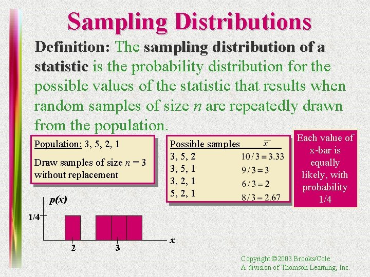
Sampling Distributions Definition: The sampling distribution of a statistic is the probability distribution for the possible values of the statistic that results when random samples of size n are repeatedly drawn from the population. Population: 3, 5, 2, 1 Draw samples of size n = 3 without replacement p(x) Possible samples 3, 5, 2 3, 5, 1 3, 2, 1 5, 2, 1 Each value of x-bar is equally likely, with probability 1/4 2 3 x Copyright © 2003 Brooks/Cole A division of Thomson Learning, Inc.
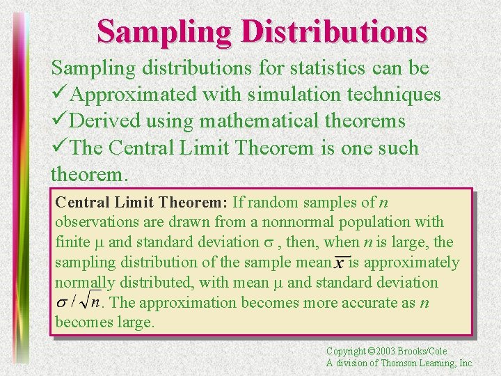
Sampling Distributions Sampling distributions for statistics can be üApproximated with simulation techniques üDerived using mathematical theorems üThe Central Limit Theorem is one such theorem. Central Limit Theorem: If random samples of n observations are drawn from a nonnormal population with finite m and standard deviation s , then, when n is large, the sampling distribution of the sample mean is approximately normally distributed, with mean m and standard deviation. The approximation becomes more accurate as n becomes large. Copyright © 2003 Brooks/Cole A division of Thomson Learning, Inc.
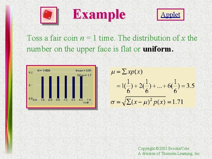
Example Applet Toss a fair coin n = 1 time. The distribution of x the number on the upper face is flat or uniform. Copyright © 2003 Brooks/Cole A division of Thomson Learning, Inc.
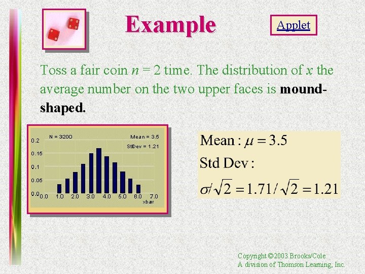
Example Applet Toss a fair coin n = 2 time. The distribution of x the average number on the two upper faces is moundshaped. Copyright © 2003 Brooks/Cole A division of Thomson Learning, Inc.
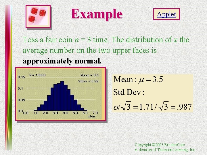
Example Applet Toss a fair coin n = 3 time. The distribution of x the average number on the two upper faces is approximately normal. Copyright © 2003 Brooks/Cole A division of Thomson Learning, Inc.
Why is this Important? üThe Central Limit Theorem also implies that the sum of n measurements is approximately normal with mean nm and standard deviation. üMany statistics that are used for statistical inference are sums or averages of sample measurements. üWhen n is large, these statistics will have approximately normal distributions. üThis will allow us to describe their behavior and evaluate the reliability of our inferences. Copyright © 2003 Brooks/Cole A division of Thomson Learning, Inc.
How Large is Large? If the sample is normal, normal then the sampling distribution of will also be normal, no matter what the sample size. When the sample population is approximately symmetric, symmetric the distribution becomes approximately normal for relatively small values of n. When the sample population is skewed, skewed the sample size must be at least 30 before the sampling distribution of becomes approximately normal. Copyright © 2003 Brooks/Cole A division of Thomson Learning, Inc.
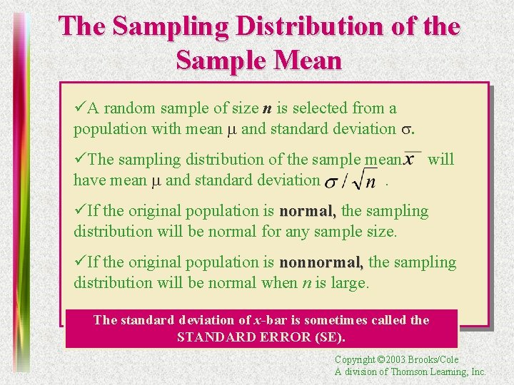
The Sampling Distribution of the Sample Mean üA random sample of size n is selected from a population with mean m and standard deviation s. üThe sampling distribution of the sample mean have mean m and standard deviation. will üIf the original population is normal, the sampling distribution will be normal for any sample size. üIf the original population is nonnormal, the sampling distribution will be normal when n is large. The standard deviation of x-bar is sometimes called the STANDARD ERROR (SE). Copyright © 2003 Brooks/Cole A division of Thomson Learning, Inc.
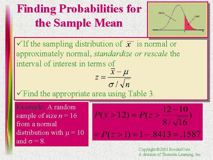
Finding Probabilities for the Sample Mean üIf the sampling distribution of is normal or approximately normal, standardize or rescale the interval of interest in terms of üFind the appropriate area using Table 3. Example: A random sample of size n = 16 from a normal distribution with m = 10 and s = 8. Copyright © 2003 Brooks/Cole A division of Thomson Learning, Inc.
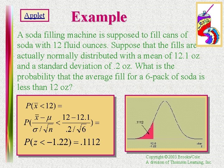
Applet Example A soda filling machine is supposed to fill cans of soda with 12 fluid ounces. Suppose that the fills are actually normally distributed with a mean of 12. 1 oz and a standard deviation of. 2 oz. What is the probability that the average fill for a 6 -pack of soda is less than 12 oz? Copyright © 2003 Brooks/Cole A division of Thomson Learning, Inc.
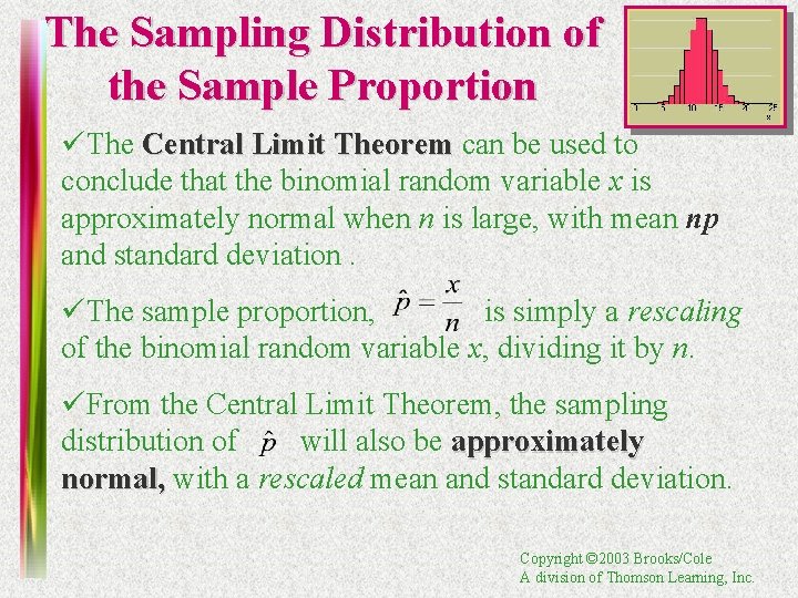
The Sampling Distribution of the Sample Proportion üThe Central Limit Theorem can be used to conclude that the binomial random variable x is approximately normal when n is large, with mean np and standard deviation. üThe sample proportion, is simply a rescaling of the binomial random variable x, dividing it by n. üFrom the Central Limit Theorem, the sampling distribution of will also be approximately normal, with a rescaled mean and standard deviation. Copyright © 2003 Brooks/Cole A division of Thomson Learning, Inc.
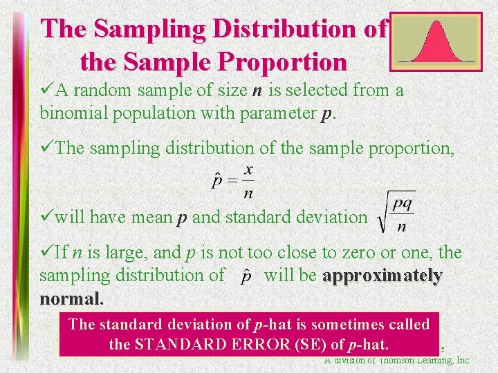
The Sampling Distribution of the Sample Proportion üA random sample of size n is selected from a binomial population with parameter p. üThe sampling distribution of the sample proportion, üwill have mean p and standard deviation üIf n is large, and p is not too close to zero or one, the sampling distribution of will be approximately normal. The standard deviation of p-hat is sometimes called the STANDARD ERROR (SE)Copyright of p-hat. © 2003 Brooks/Cole A division of Thomson Learning, Inc.
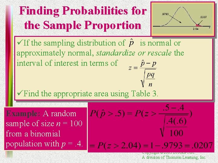
Finding Probabilities for the Sample Proportion üIf the sampling distribution of is normal or approximately normal, standardize or rescale the interval of interest in terms of üFind the appropriate area using Table 3. Example: A random sample of size n = 100 from a binomial population with p =. 4. Copyright © 2003 Brooks/Cole A division of Thomson Learning, Inc.
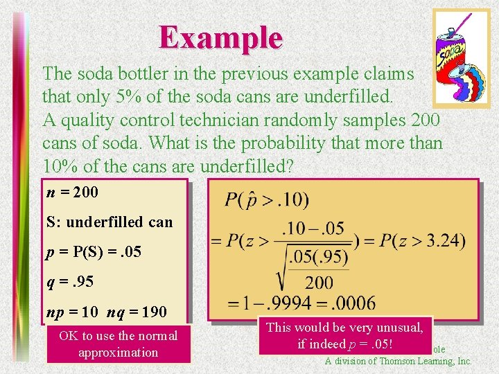
Example The soda bottler in the previous example claims that only 5% of the soda cans are underfilled. A quality control technician randomly samples 200 cans of soda. What is the probability that more than 10% of the cans are underfilled? n = 200 S: underfilled can p = P(S) =. 05 q =. 95 np = 10 nq = 190 OK to use the normal approximation This would be very unusual, if indeed p =© 2003. 05! Brooks/Cole Copyright A division of Thomson Learning, Inc.
Types of Inference • Estimation: – Estimating or predicting the value of the parameter – “What is (are) the most likely values of m or p? ” • Hypothesis Testing: – Deciding about the value of a parameter based on some preconceived idea. – “Did the sample come from a population with m = 5 or p =. 2? ” Copyright © 2003 Brooks/Cole A division of Thomson Learning, Inc.
Types of Inference • Examples: – A consumer wants to estimate the average price of similar homes in her city before putting her home on the market. Estimation: Estimate m, the average home price. –A manufacturer wants to know if a new type of steel is more resistant to high temperatures than an old type was. Hypothesis test: test Is the new average resistance, m. N equal to the old average resistance, m. O? Copyright © 2003 Brooks/Cole A division of Thomson Learning, Inc.
Definitions • An estimator is a rule, usually a formula, that tells you how to calculate the estimate based on the sample. – Point estimation: A single number is calculated to estimate the parameter. – Interval estimation: Two numbers are calculated to create an interval within which the parameter is expected to lie. Copyright © 2003 Brooks/Cole A division of Thomson Learning, Inc.
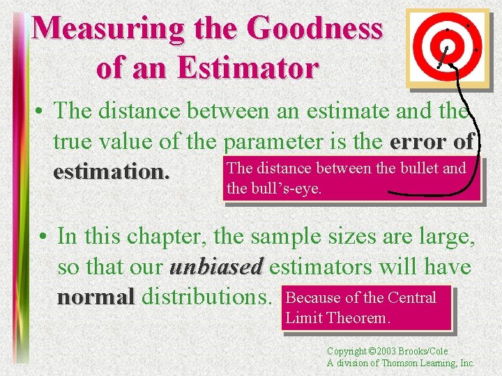
Measuring the Goodness of an Estimator • The distance between an estimate and the true value of the parameter is the error of The distance between the bullet and estimation. the bull’s-eye. • In this chapter, the sample sizes are large, so that our unbiased estimators will have normal distributions. Because of the Central Limit Theorem. Copyright © 2003 Brooks/Cole A division of Thomson Learning, Inc.
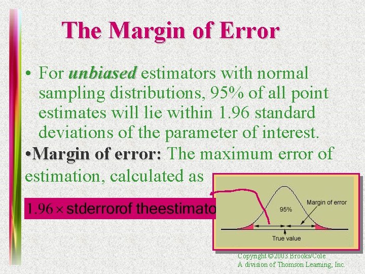
The Margin of Error • For unbiased estimators with normal sampling distributions, 95% of all point estimates will lie within 1. 96 standard deviations of the parameter of interest. • Margin of error: The maximum error of estimation, calculated as Copyright © 2003 Brooks/Cole A division of Thomson Learning, Inc.
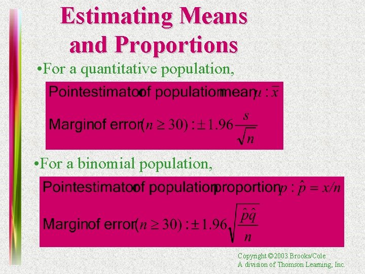
Estimating Means and Proportions • For a quantitative population, • For a binomial population, Copyright © 2003 Brooks/Cole A division of Thomson Learning, Inc.
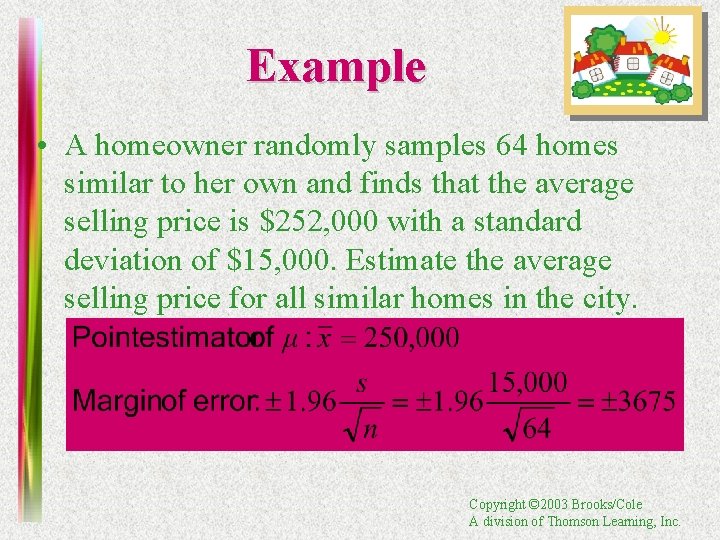
Example • A homeowner randomly samples 64 homes similar to her own and finds that the average selling price is $252, 000 with a standard deviation of $15, 000. Estimate the average selling price for all similar homes in the city. Copyright © 2003 Brooks/Cole A division of Thomson Learning, Inc.
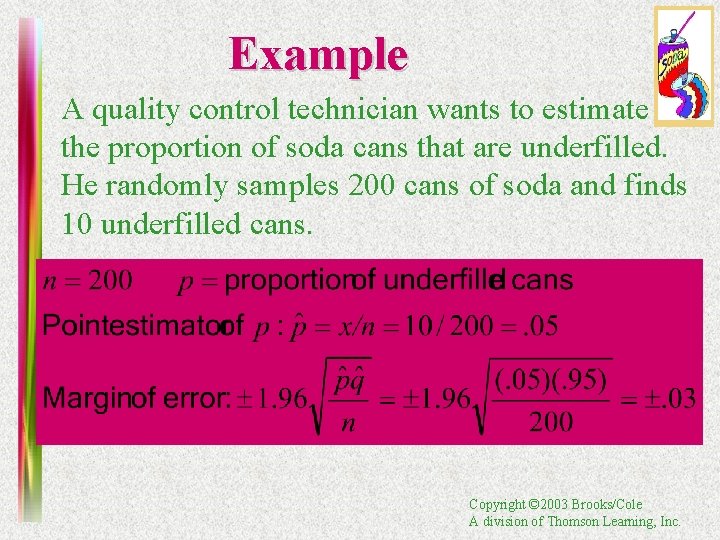
Example A quality control technician wants to estimate the proportion of soda cans that are underfilled. He randomly samples 200 cans of soda and finds 10 underfilled cans. Copyright © 2003 Brooks/Cole A division of Thomson Learning, Inc.
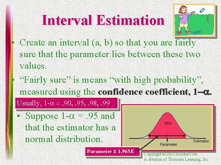
Interval Estimation • Create an interval (a, b) so that you are fairly sure that the parameter lies between these two values. • “Fairly sure” is means “with high probability”, measured using the confidence coefficient, 1 -a. Usually, 1 -a =. 90, . 95, . 98, . 99 • Suppose 1 -a =. 95 and that the estimator has a normal distribution. Parameter 1. 96 SE Copyright © 2003 Brooks/Cole A division of Thomson Learning, Inc.
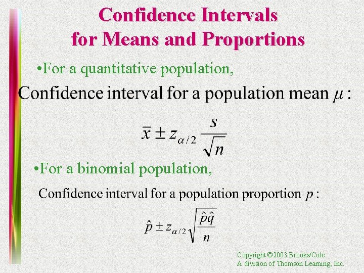
Confidence Intervals for Means and Proportions • For a quantitative population, • For a binomial population, Copyright © 2003 Brooks/Cole A division of Thomson Learning, Inc.
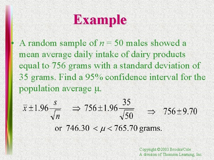
Example • A random sample of n = 50 males showed a mean average daily intake of dairy products equal to 756 grams with a standard deviation of 35 grams. Find a 95% confidence interval for the population average m. Copyright © 2003 Brooks/Cole A division of Thomson Learning, Inc.
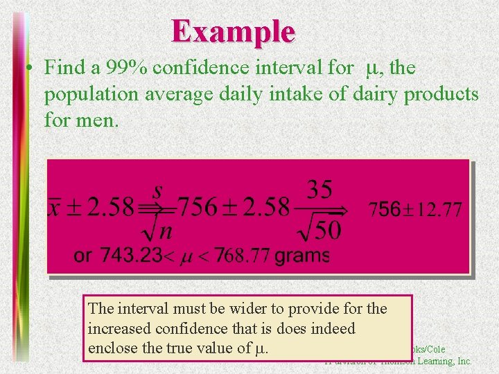
Example • Find a 99% confidence interval for m, the population average daily intake of dairy products for men. The interval must be wider to provide for the increased confidence that is does indeed Copyright © 2003 Brooks/Cole enclose the true value of m. A division of Thomson Learning, Inc.
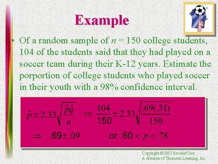
Example • Of a random sample of n = 150 college students, 104 of the students said that they had played on a soccer team during their K-12 years. Estimate the porportion of college students who played soccer in their youth with a 98% confidence interval. Copyright © 2003 Brooks/Cole A division of Thomson Learning, Inc.
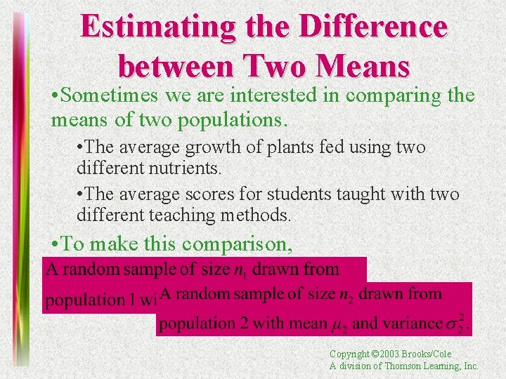
Estimating the Difference between Two Means • Sometimes we are interested in comparing the means of two populations. • The average growth of plants fed using two different nutrients. • The average scores for students taught with two different teaching methods. • To make this comparison, Copyright © 2003 Brooks/Cole A division of Thomson Learning, Inc.
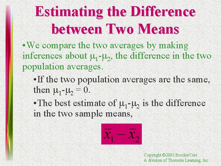
Estimating the Difference between Two Means • We compare the two averages by making inferences about m 1 -m 2, the difference in the two population averages. • If the two population averages are the same, then m 1 -m 2 = 0. • The best estimate of m 1 -m 2 is the difference in the two sample means, Copyright © 2003 Brooks/Cole A division of Thomson Learning, Inc.
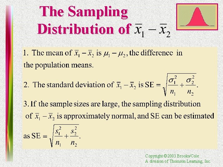
The Sampling Distribution of Copyright © 2003 Brooks/Cole A division of Thomson Learning, Inc.
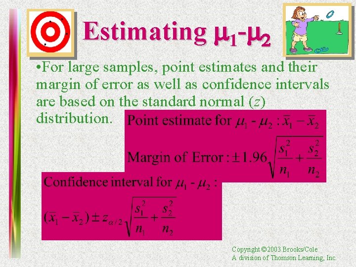
Estimating m 1 -m 2 • For large samples, point estimates and their margin of error as well as confidence intervals are based on the standard normal (z) distribution. Copyright © 2003 Brooks/Cole A division of Thomson Learning, Inc.
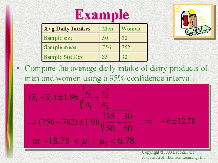
Example Avg Daily Intakes Men Women Sample size 50 50 Sample mean 756 762 Sample Std Dev 35 30 • Compare the average daily intake of dairy products of men and women using a 95% confidence interval. Copyright © 2003 Brooks/Cole A division of Thomson Learning, Inc.
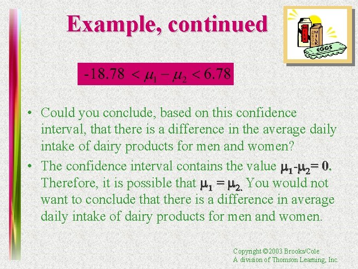
Example, continued • Could you conclude, based on this confidence interval, that there is a difference in the average daily intake of dairy products for men and women? • The confidence interval contains the value m 1 -m 2= 0. Therefore, it is possible that m 1 = m 2. You would not want to conclude that there is a difference in average daily intake of dairy products for men and women. Copyright © 2003 Brooks/Cole A division of Thomson Learning, Inc.
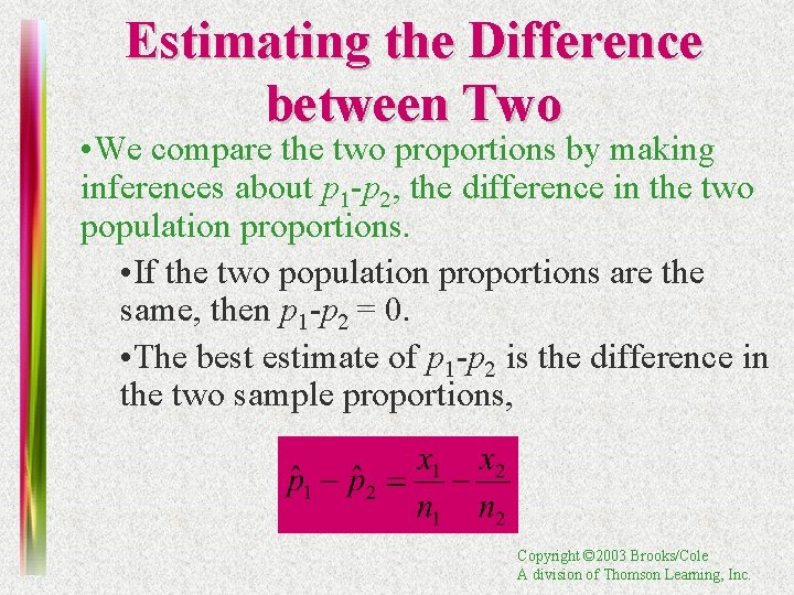
Estimating the Difference between Two • We compare the two proportions by making inferences about p 1 -p 2, the difference in the two population proportions. • If the two population proportions are the same, then p 1 -p 2 = 0. • The best estimate of p 1 -p 2 is the difference in the two sample proportions, Copyright © 2003 Brooks/Cole A division of Thomson Learning, Inc.
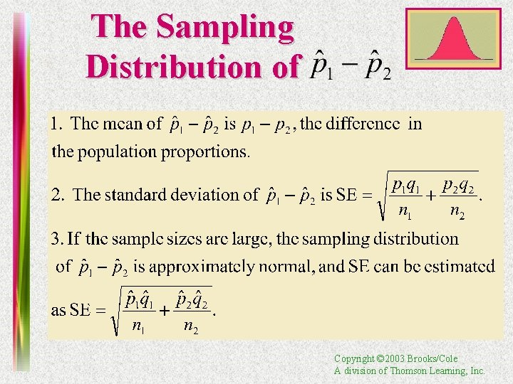
The Sampling Distribution of Copyright © 2003 Brooks/Cole A division of Thomson Learning, Inc.
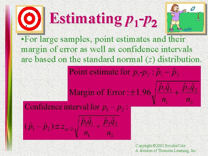
Estimating p 1 -p 2 • For large samples, point estimates and their margin of error as well as confidence intervals are based on the standard normal (z) distribution. Copyright © 2003 Brooks/Cole A division of Thomson Learning, Inc.
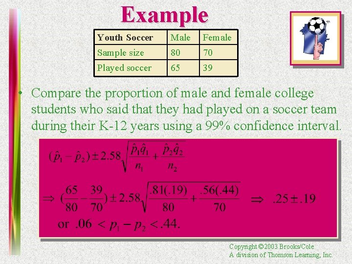
Example Youth Soccer Male Female Sample size 80 70 Played soccer 65 39 • Compare the proportion of male and female college students who said that they had played on a soccer team during their K-12 years using a 99% confidence interval. Copyright © 2003 Brooks/Cole A division of Thomson Learning, Inc.
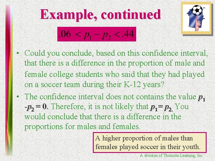
Example, continued • Could you conclude, based on this confidence interval, that there is a difference in the proportion of male and female college students who said that they had played on a soccer team during their K-12 years? • The confidence interval does not contains the value p 1 -p 2 = 0. Therefore, it is not likely that p 1= p 2. You would conclude that there is a difference in the proportions for males and females. A higher proportion of males than females played Copyright soccer© 2003 in their youth. Brooks/Cole A division of Thomson Learning, Inc.
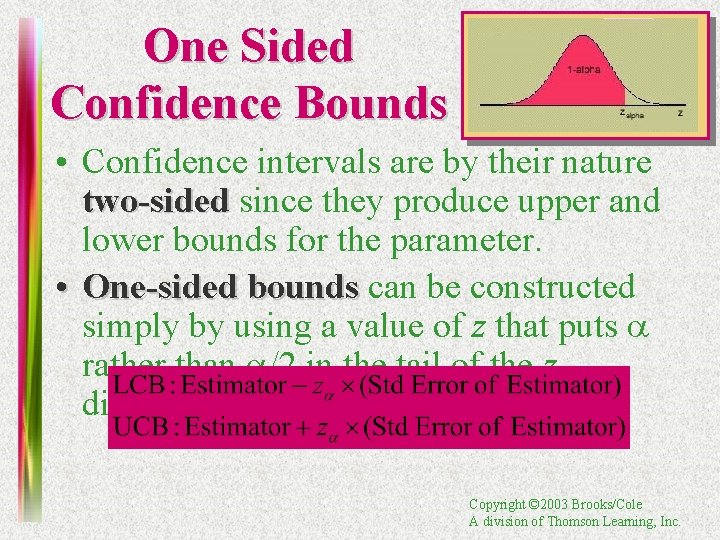
One Sided Confidence Bounds • Confidence intervals are by their nature two-sided since they produce upper and lower bounds for the parameter. • One-sided bounds can be constructed simply by using a value of z that puts a rather than a/2 in the tail of the z distribution. Copyright © 2003 Brooks/Cole A division of Thomson Learning, Inc.
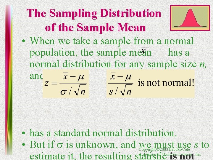
The Sampling Distribution of the Sample Mean • When we take a sample from a normal population, the sample mean has a normal distribution for any sample size n, and • has a standard normal distribution. • But if s is unknown, and we must use s to estimate it, the resulting statistic is not Copyright © 2003 Brooks/Cole A division of Thomson Learning, Inc.
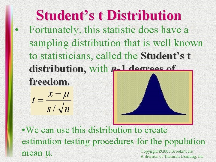
Student’s t Distribution • Fortunately, this statistic does have a sampling distribution that is well known to statisticians, called the Student’s t distribution, with n-1 degrees of freedom. • We can use this distribution to create estimation testing procedures for the population Copyright © 2003 Brooks/Cole mean m. A division of Thomson Learning, Inc.
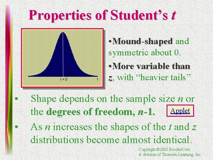
Properties of Student’s t • Mound-shaped and symmetric about 0. • More variable than z, with “heavier tails” • • Shape depends on the sample size n or the degrees of freedom, n-1. Applet As n increases the shapes of the t and z distributions become almost identical. Copyright © 2003 Brooks/Cole A division of Thomson Learning, Inc.
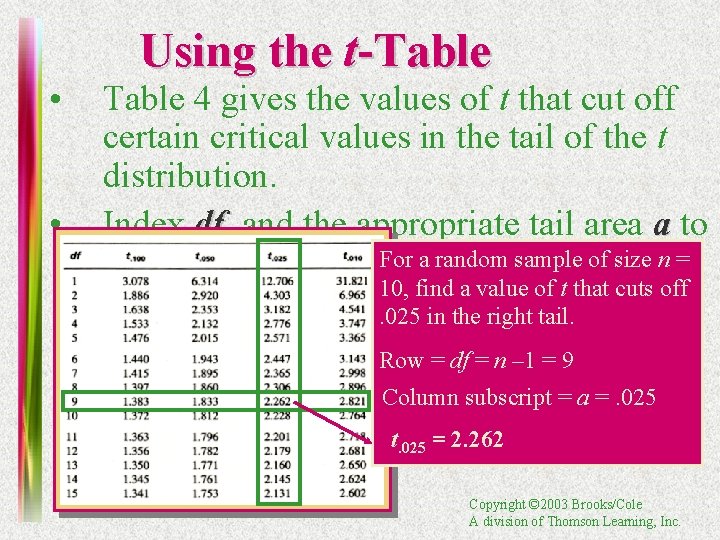
• • Using the t-Table 4 gives the values of t that cut off certain critical values in the tail of the t distribution. Index df and the appropriate tail area a to a random size n = find ta, the value of For t with areasample a toofits 10, find a value of t that cuts off right. . 025 in the right tail. Row = df = n – 1 = 9 Column subscript = a =. 025 t. 025 = 2. 262 Copyright © 2003 Brooks/Cole A division of Thomson Learning, Inc.
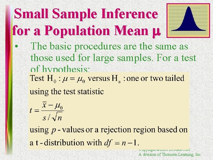
Small Sample Inference for a Population Mean m • The basic procedures are the same as those used for large samples. For a test of hypothesis: Copyright © 2003 Brooks/Cole A division of Thomson Learning, Inc.
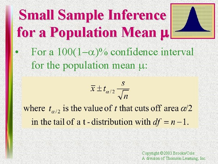
Small Sample Inference for a Population Mean m • For a 100(1 -a)% confidence interval for the population mean m: Copyright © 2003 Brooks/Cole A division of Thomson Learning, Inc.
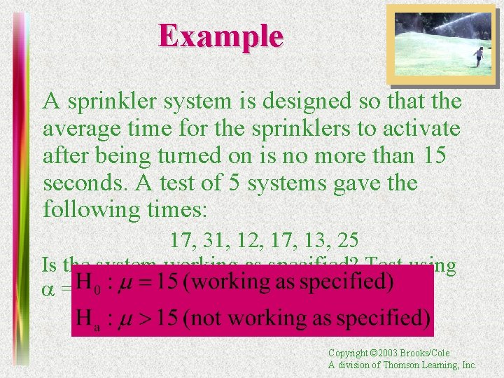
Example A sprinkler system is designed so that the average time for the sprinklers to activate after being turned on is no more than 15 seconds. A test of 5 systems gave the following times: 17, 31, 12, 17, 13, 25 Is the system working as specified? Test using a =. 05. Copyright © 2003 Brooks/Cole A division of Thomson Learning, Inc.
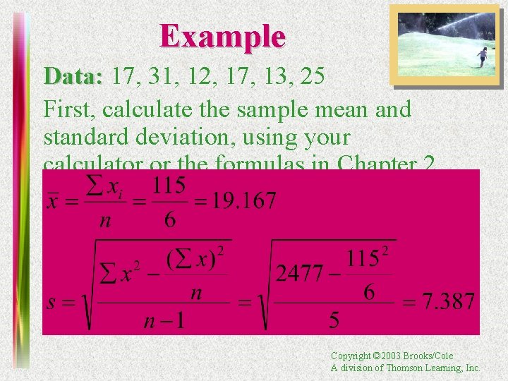
Example Data: 17, 31, 12, 17, 13, 25 First, calculate the sample mean and standard deviation, using your calculator or the formulas in Chapter 2. Copyright © 2003 Brooks/Cole A division of Thomson Learning, Inc.
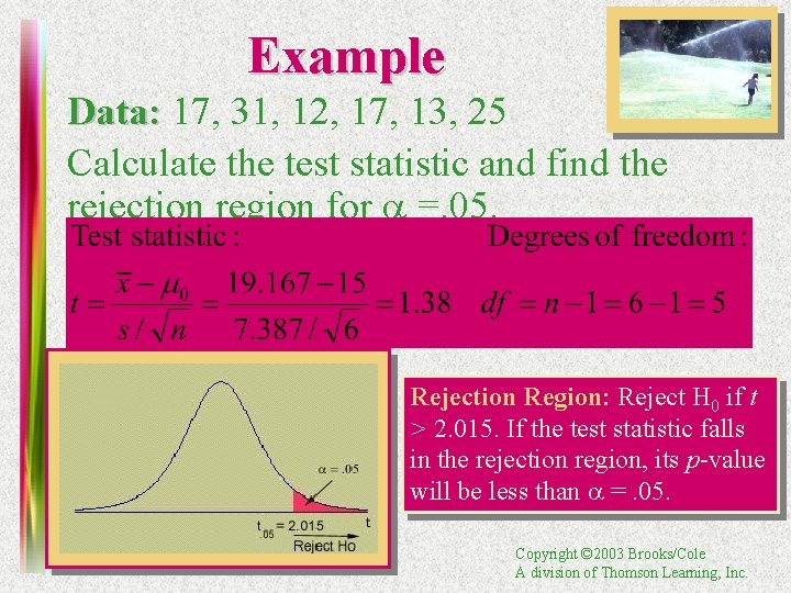
Example Data: 17, 31, 12, 17, 13, 25 Calculate the test statistic and find the rejection region for a =. 05. Rejection Region: Reject H 0 if t > 2. 015. If the test statistic falls in the rejection region, its p-value will be less than a =. 05. Copyright © 2003 Brooks/Cole A division of Thomson Learning, Inc.
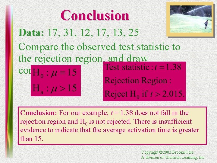
Conclusion Data: 17, 31, 12, 17, 13, 25 Compare the observed test statistic to the rejection region, and draw conclusions. Conclusion: For our example, t = 1. 38 does not fall in the rejection region and H 0 is not rejected. There is insufficient evidence to indicate that the average activation time is greater than 15. Copyright © 2003 Brooks/Cole A division of Thomson Learning, Inc.
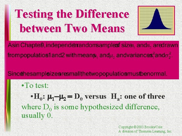
Testing the Difference between Two Means • To test: • H 0: m 1 -m 2 = D 0 versus Ha: one of three where D 0 is some hypothesized difference, usually 0. Copyright © 2003 Brooks/Cole A division of Thomson Learning, Inc.
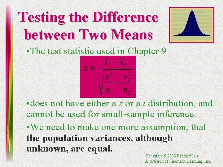
Testing the Difference between Two Means • The test statistic used in Chapter 9 • does not have either a z or a t distribution, and cannot be used for small-sample inference. • We need to make one more assumption, that the population variances, although unknown, are equal. Copyright © 2003 Brooks/Cole A division of Thomson Learning, Inc.
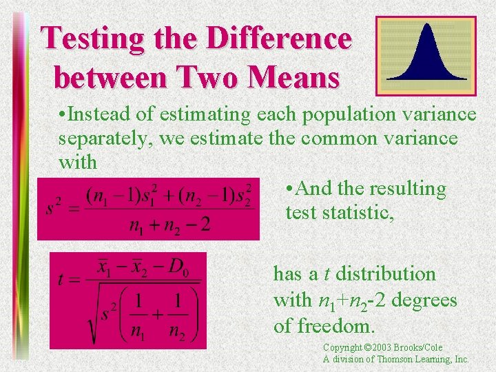
Testing the Difference between Two Means • Instead of estimating each population variance separately, we estimate the common variance with • And the resulting test statistic, has a t distribution with n 1+n 2 -2 degrees of freedom. Copyright © 2003 Brooks/Cole A division of Thomson Learning, Inc.
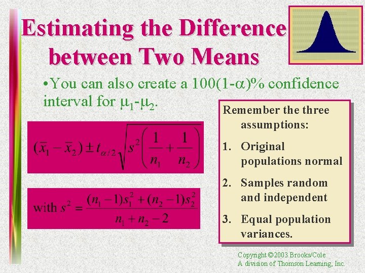
Estimating the Difference between Two Means • You can also create a 100(1 -a)% confidence interval for m 1 -m 2. Remember the three assumptions: 1. Original populations normal 2. Samples random and independent 3. Equal population variances. Copyright © 2003 Brooks/Cole A division of Thomson Learning, Inc.
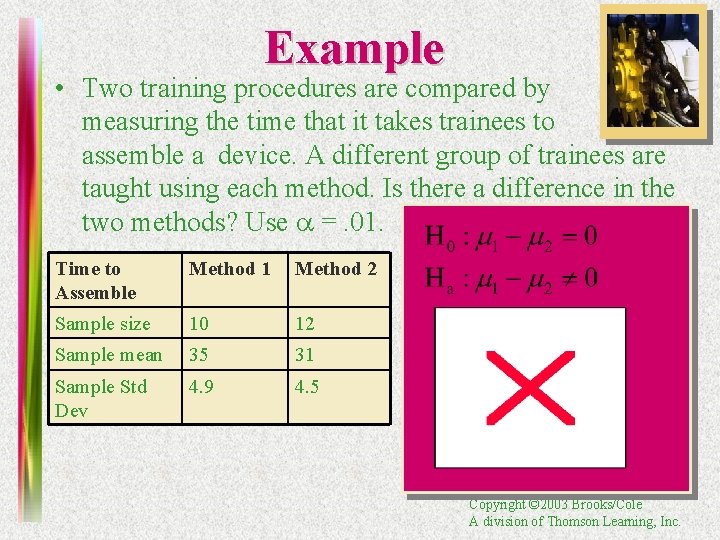
Example • Two training procedures are compared by measuring the time that it takes trainees to assemble a device. A different group of trainees are taught using each method. Is there a difference in the two methods? Use a =. 01. Time to Assemble Method 1 Method 2 Sample size 10 12 Sample mean 35 31 Sample Std Dev 4. 9 4. 5 Copyright © 2003 Brooks/Cole A division of Thomson Learning, Inc.
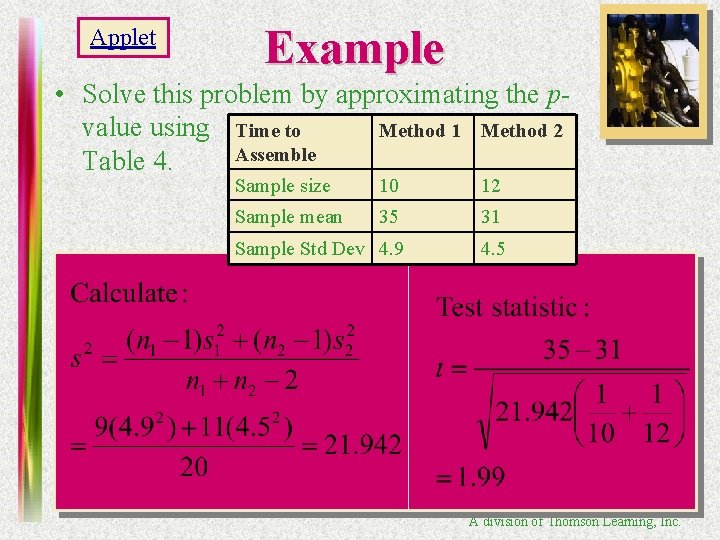
Applet Example • Solve this problem by approximating the pvalue using Time to Method 1 Method 2 Assemble Table 4. Sample size 10 12 Sample mean 35 31 Sample Std Dev 4. 9 4. 5 Copyright © 2003 Brooks/Cole A division of Thomson Learning, Inc.
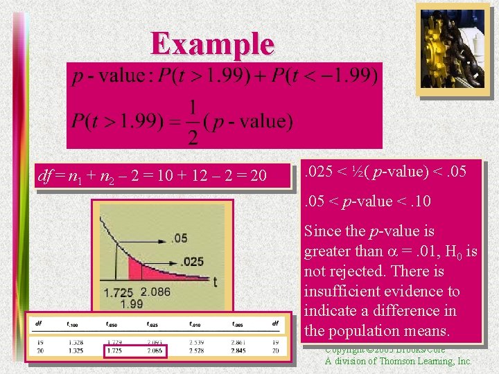
Example df = n 1 + n 2 – 2 = 10 + 12 – 2 = 20 . 025 < ½( p-value) <. 05 < p-value <. 10 Since the p-value is greater than a =. 01, H 0 is not rejected. There is insufficient evidence to indicate a difference in the population means. Copyright © 2003 Brooks/Cole A division of Thomson Learning, Inc.
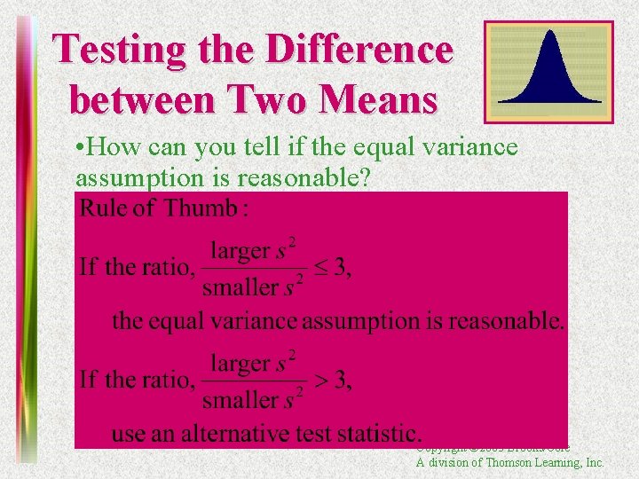
Testing the Difference between Two Means • How can you tell if the equal variance assumption is reasonable? Copyright © 2003 Brooks/Cole A division of Thomson Learning, Inc.
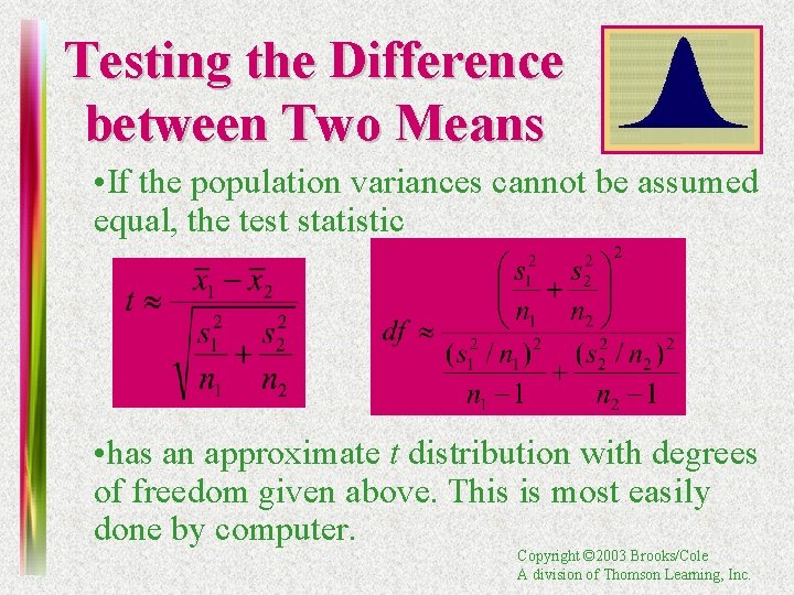
Testing the Difference between Two Means • If the population variances cannot be assumed equal, the test statistic • has an approximate t distribution with degrees of freedom given above. This is most easily done by computer. Copyright © 2003 Brooks/Cole A division of Thomson Learning, Inc.
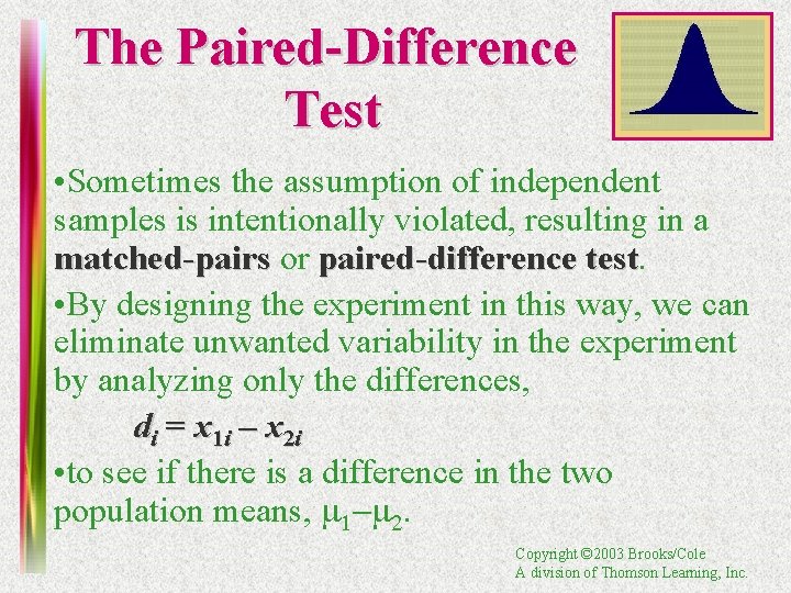
The Paired-Difference Test • Sometimes the assumption of independent samples is intentionally violated, resulting in a matched-pairs or paired-difference test • By designing the experiment in this way, we can eliminate unwanted variability in the experiment by analyzing only the differences, di = x 1 i – x 2 i • to see if there is a difference in the two population means, m 1 -m 2. Copyright © 2003 Brooks/Cole A division of Thomson Learning, Inc.
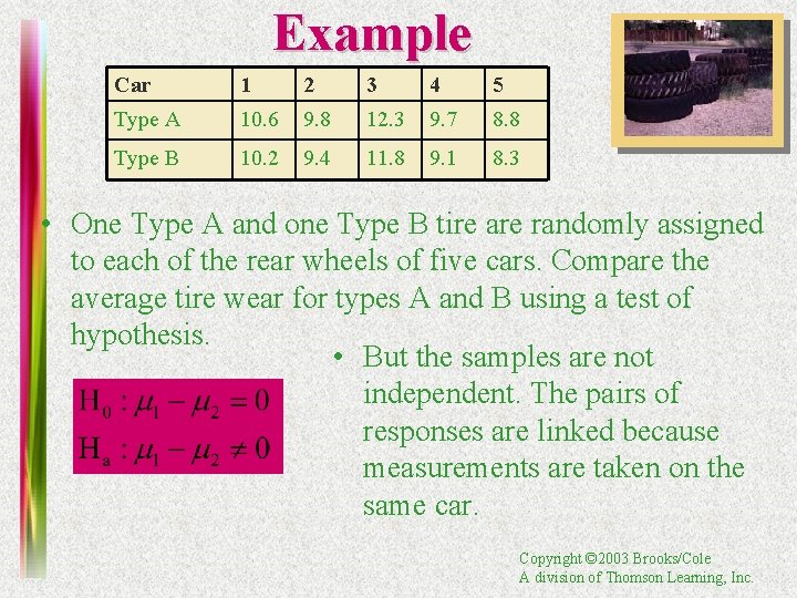
Example Car 1 2 3 4 5 Type A 10. 6 9. 8 12. 3 9. 7 8. 8 Type B 10. 2 9. 4 11. 8 9. 1 8. 3 • One Type A and one Type B tire are randomly assigned to each of the rear wheels of five cars. Compare the average tire wear for types A and B using a test of hypothesis. • But the samples are not independent. The pairs of responses are linked because measurements are taken on the same car. Copyright © 2003 Brooks/Cole A division of Thomson Learning, Inc.
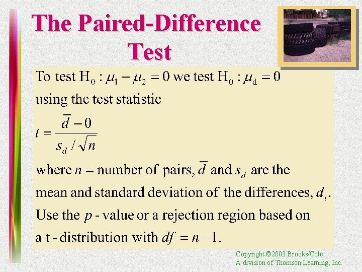
The Paired-Difference Test Copyright © 2003 Brooks/Cole A division of Thomson Learning, Inc.
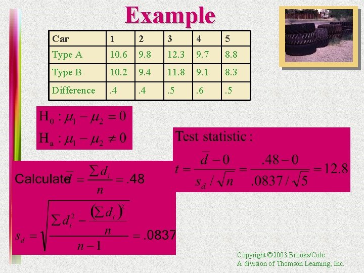
Example Car 1 2 3 4 5 Type A 10. 6 9. 8 12. 3 9. 7 8. 8 Type B 10. 2 9. 4 11. 8 9. 1 8. 3 Difference . 4 . 5 . 6 . 5 Copyright © 2003 Brooks/Cole A division of Thomson Learning, Inc.
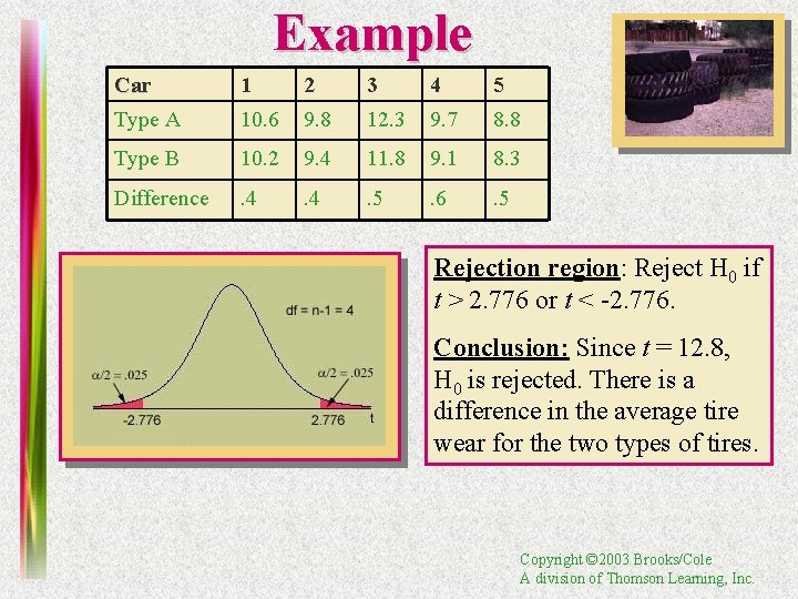
Example Car 1 2 3 4 5 Type A 10. 6 9. 8 12. 3 9. 7 8. 8 Type B 10. 2 9. 4 11. 8 9. 1 8. 3 Difference . 4 . 5 . 6 . 5 Rejection region: Reject H 0 if t > 2. 776 or t < -2. 776. Conclusion: Since t = 12. 8, H 0 is rejected. There is a difference in the average tire wear for the two types of tires. Copyright © 2003 Brooks/Cole A division of Thomson Learning, Inc.
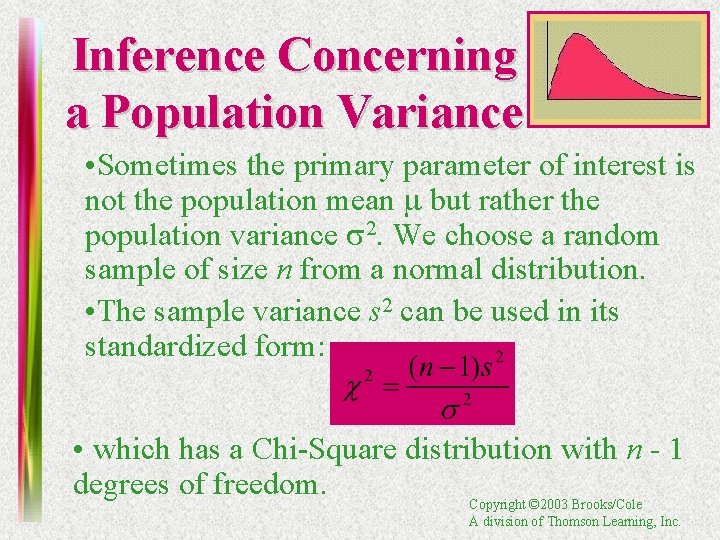
Inference Concerning a Population Variance • Sometimes the primary parameter of interest is not the population mean m but rather the population variance s 2. We choose a random sample of size n from a normal distribution. • The sample variance s 2 can be used in its standardized form: • which has a Chi-Square distribution with n - 1 degrees of freedom. Copyright © 2003 Brooks/Cole A division of Thomson Learning, Inc.
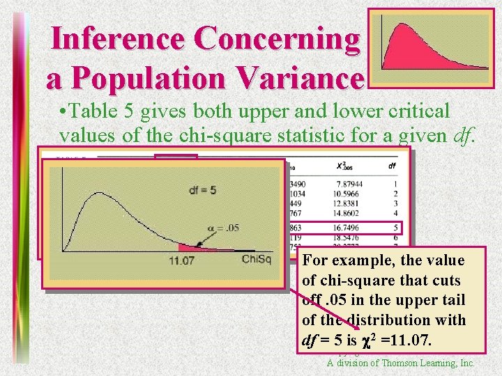
Inference Concerning a Population Variance • Table 5 gives both upper and lower critical values of the chi-square statistic for a given df. For example, the value of chi-square that cuts off. 05 in the upper tail of the distribution with df = 5 is c 2 =11. 07. Copyright © 2003 Brooks/Cole A division of Thomson Learning, Inc.
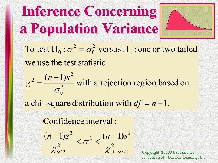
Inference Concerning a Population Variance Copyright © 2003 Brooks/Cole A division of Thomson Learning, Inc.
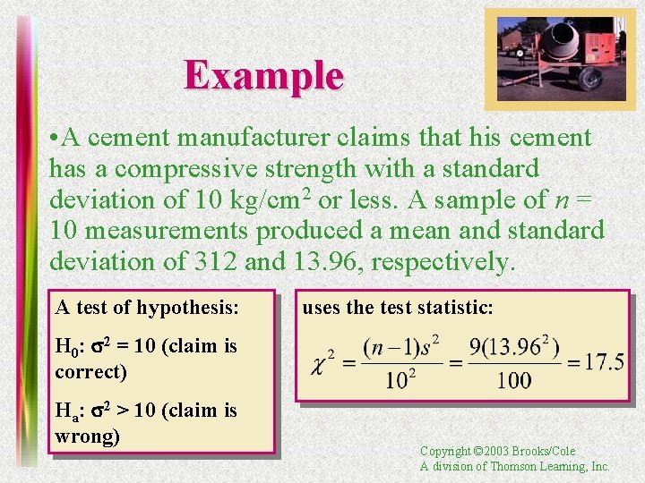
Example • A cement manufacturer claims that his cement has a compressive strength with a standard deviation of 10 kg/cm 2 or less. A sample of n = 10 measurements produced a mean and standard deviation of 312 and 13. 96, respectively. A test of hypothesis: uses the test statistic: H 0: s 2 = 10 (claim is correct) Ha: s 2 > 10 (claim is wrong) Copyright © 2003 Brooks/Cole A division of Thomson Learning, Inc.
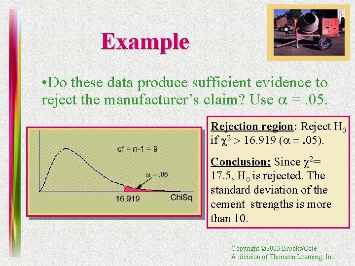
Example • Do these data produce sufficient evidence to reject the manufacturer’s claim? Use a =. 05. Rejection region: Reject H 0 if c 2 > 16. 919 (a =. 05). Conclusion: Since c 2= 17. 5, H 0 is rejected. The standard deviation of the cement strengths is more than 10. Copyright © 2003 Brooks/Cole A division of Thomson Learning, Inc.
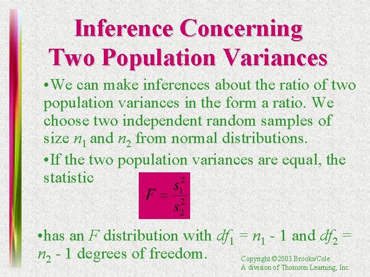
Inference Concerning Two Population Variances • We can make inferences about the ratio of two population variances in the form a ratio. We choose two independent random samples of size n 1 and n 2 from normal distributions. • If the two population variances are equal, the statistic • has an F distribution with df 1 = n 1 - 1 and df 2 = n 2 - 1 degrees of freedom. Copyright © 2003 Brooks/Cole A division of Thomson Learning, Inc.
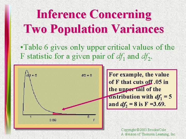
Inference Concerning Two Population Variances • Table 6 gives only upper critical values of the F statistic for a given pair of df 1 and df 2. For example, the value of F that cuts off. 05 in the upper tail of the distribution with df 1 = 5 and df 2 = 8 is F =3. 69. Copyright © 2003 Brooks/Cole A division of Thomson Learning, Inc.
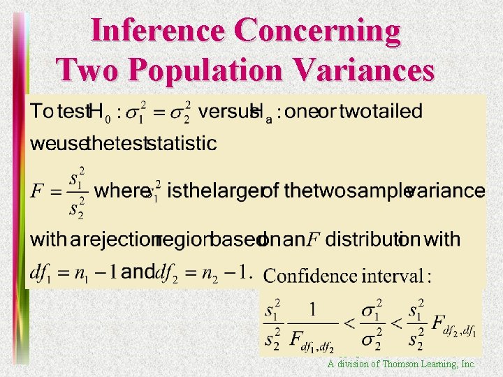
Inference Concerning Two Population Variances Copyright © 2003 Brooks/Cole A division of Thomson Learning, Inc.
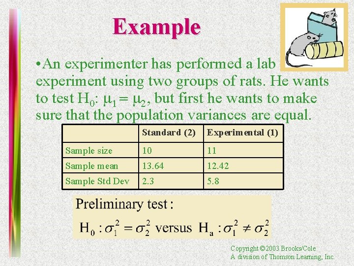
Example • An experimenter has performed a lab experiment using two groups of rats. He wants to test H 0: m 1 = m 2, but first he wants to make sure that the population variances are equal. Standard (2) Experimental (1) Sample size 10 11 Sample mean 13. 64 12. 42 Sample Std Dev 2. 3 5. 8 Copyright © 2003 Brooks/Cole A division of Thomson Learning, Inc.
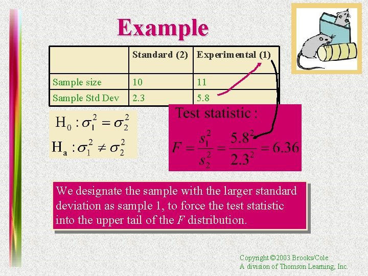
Example Standard (2) Experimental (1) Sample size 10 11 Sample Std Dev 2. 3 5. 8 We designate the sample with the larger standard deviation as sample 1, to force the test statistic into the upper tail of the F distribution. Copyright © 2003 Brooks/Cole A division of Thomson Learning, Inc.
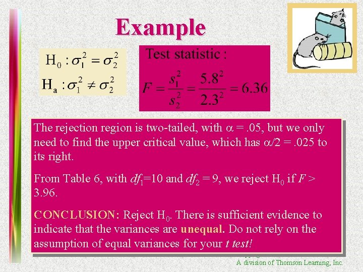
Example The rejection region is two-tailed, with a =. 05, but we only need to find the upper critical value, which has a/2 =. 025 to its right. From Table 6, with df 1=10 and df 2 = 9, we reject H 0 if F > 3. 96. CONCLUSION: Reject H 0. There is sufficient evidence to indicate that the variances are unequal. Do not rely on the assumption of equal variances for your t test! Copyright © 2003 Brooks/Cole A division of Thomson Learning, Inc.
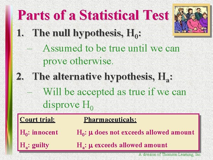
Parts of a Statistical Test 1. The null hypothesis, H 0: – Assumed to be true until we can prove otherwise. 2. The alternative hypothesis, Ha: – Will be accepted as true if we can disprove H 0 Court trial: Pharmaceuticals: H 0: innocent H 0: m does not exceeds allowed amount Ha: guilty Ha: m exceeds allowed amount Copyright © 2003 Brooks/Cole A division of Thomson Learning, Inc.
Parts of a Statistical Test 3. The test statistic and its p-value: • A single statistic calculated from the sample which will allow us to reject or not reject H 0, and • A probability, calculated from the test statistic that measures whether the test statistic is likely or unlikely, assuming H 0 is true. 4. The rejection region: – A rule that tells us for which values of the Copyright © 2003 Brooks/Cole division of Thomsonthe Learning, Inc. test statistic, or for which Ap-values, null
Parts of a Statistical Test 5. Conclusion: – Either “Reject H 0” or “Do not reject H 0”, along with a statement about the reliability of your conclusion. How do you decide when to reject H 0? – – Depends on the significance level, a, the maximum tolerable risk you want to have of making a mistake, if you decide to reject H 0. Usually, the significance level is a =. 01 or a =. 05. Copyright © 2003 Brooks/Cole A division of Thomson Learning, Inc.
Large Sample Test of a Population Mean, m • Take a random sample of size n 30 from a population with mean m and standard deviation s. • We assume that either 1. s is known or 2. s s since n is large • The hypothesis to be tested is – H 0: m = m 0 versus Ha: m. Copyright m 0© 2003 Brooks/Cole A division of Thomson Learning, Inc.
Test Statistic • Assume to begin with that H 0 is true. The sample mean is our best estimate of m, and we use it in a standardized form as the test statistic: since has an approximate normal distribution with mean m 0 and standard deviation. Copyright © 2003 Brooks/Cole A division of Thomson Learning, Inc.
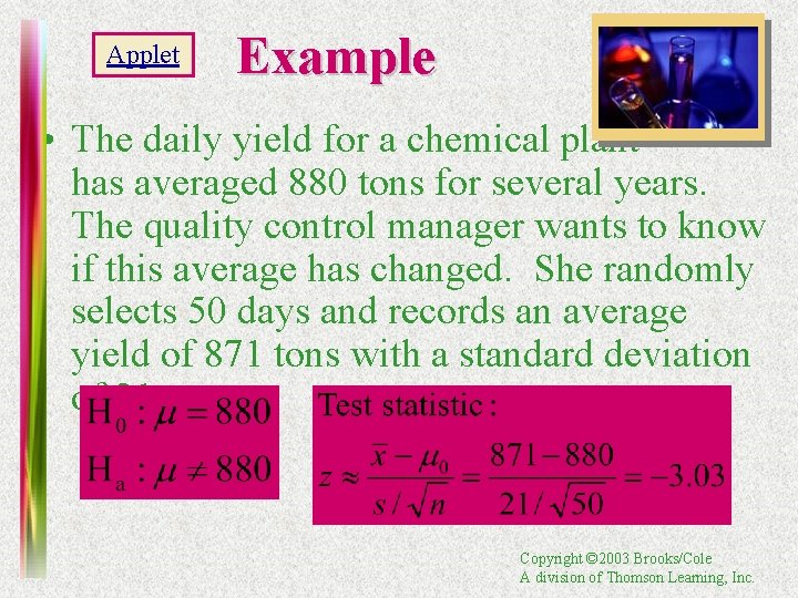
Applet Example • The daily yield for a chemical plant has averaged 880 tons for several years. The quality control manager wants to know if this average has changed. She randomly selects 50 days and records an average yield of 871 tons with a standard deviation of 21 tons. Copyright © 2003 Brooks/Cole A division of Thomson Learning, Inc.
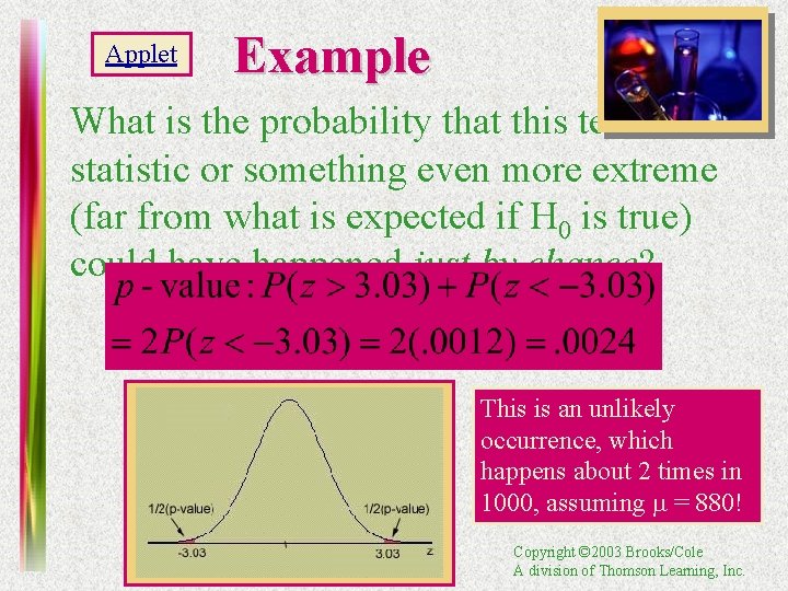
Applet Example What is the probability that this test statistic or something even more extreme (far from what is expected if H 0 is true) could have happened just by chance? This is an unlikely occurrence, which happens about 2 times in 1000, assuming m = 880! Copyright © 2003 Brooks/Cole A division of Thomson Learning, Inc.
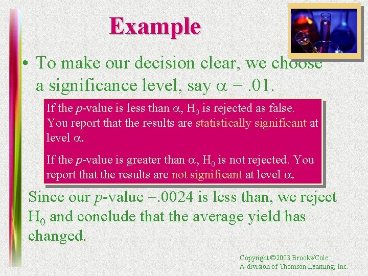
Example • To make our decision clear, we choose a significance level, say a =. 01. If the p-value is less than a, H 0 is rejected as false. You report that the results are statistically significant at level a. If the p-value is greater than a, H 0 is not rejected. You report that the results are not significant at level a. Since our p-value =. 0024 is less than, we reject H 0 and conclude that the average yield has changed. Copyright © 2003 Brooks/Cole A division of Thomson Learning, Inc.
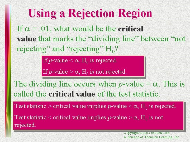
Using a Rejection Region If a =. 01, what would be the critical value that marks the “dividing line” between “not rejecting” and “rejecting” H 0? If p-value < a, H 0 is rejected. If p-value > a, H 0 is not rejected. The dividing line occurs when p-value = a. This is called the critical value of the test statistic. Test statistic > critical value implies p-value < a, H 0 is rejected. Test statistic < critical value implies p-value > a, H 0 is not rejected. Copyright © 2003 Brooks/Cole A division of Thomson Learning, Inc.
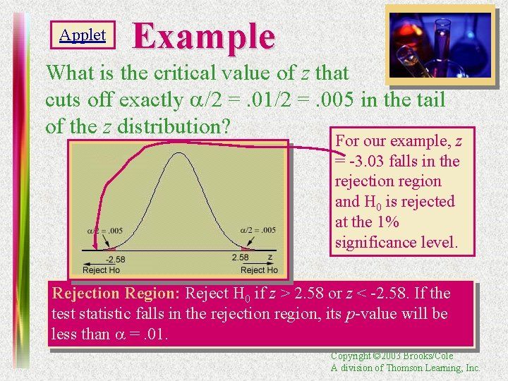
Applet Example What is the critical value of z that cuts off exactly a/2 =. 01/2 =. 005 in the tail of the z distribution? For our example, z = -3. 03 falls in the rejection region and H 0 is rejected at the 1% significance level. Rejection Region: Reject H 0 if z > 2. 58 or z < -2. 58. If the test statistic falls in the rejection region, its p-value will be less than a =. 01. Copyright © 2003 Brooks/Cole A division of Thomson Learning, Inc.
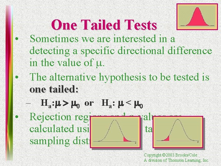
One Tailed Tests • Sometimes we are interested in a detecting a specific directional difference in the value of m. • The alternative hypothesis to be tested is one tailed: – Ha: m > m 0 or Ha: m < m 0 • Rejection regions and p-values are calculated using only one tail of the sampling distribution. Copyright © 2003 Brooks/Cole A division of Thomson Learning, Inc.
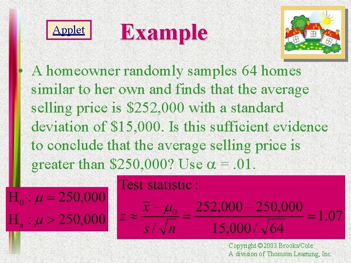
Applet Example • A homeowner randomly samples 64 homes similar to her own and finds that the average selling price is $252, 000 with a standard deviation of $15, 000. Is this sufficient evidence to conclude that the average selling price is greater than $250, 000? Use a =. 01. Copyright © 2003 Brooks/Cole A division of Thomson Learning, Inc.
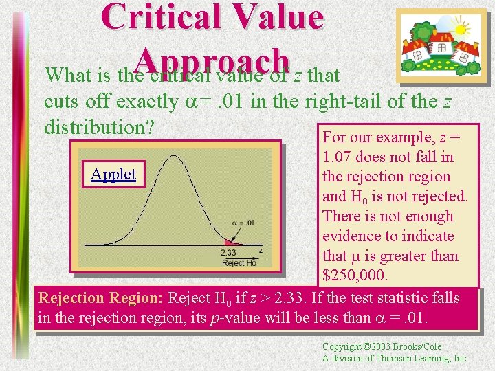
Critical Value Approach What is the critical value of z that cuts off exactly a=. 01 in the right-tail of the z distribution? For our example, z = 1. 07 does not fall in Applet the rejection region and H 0 is not rejected. There is not enough evidence to indicate that m is greater than $250, 000. Rejection Region: Reject H 0 if z > 2. 33. If the test statistic falls in the rejection region, its p-value will be less than a =. 01. Copyright © 2003 Brooks/Cole A division of Thomson Learning, Inc.
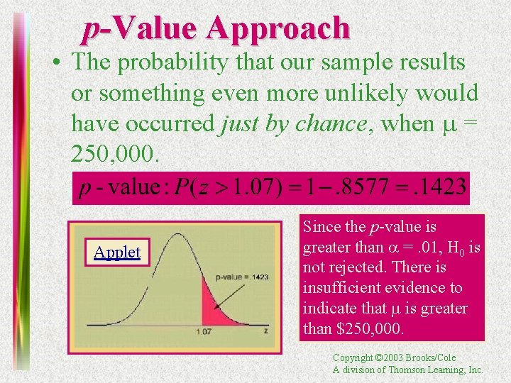
p-Value Approach • The probability that our sample results or something even more unlikely would have occurred just by chance, when m = 250, 000. Applet Since the p-value is greater than a =. 01, H 0 is not rejected. There is insufficient evidence to indicate that m is greater than $250, 000. Copyright © 2003 Brooks/Cole A division of Thomson Learning, Inc.
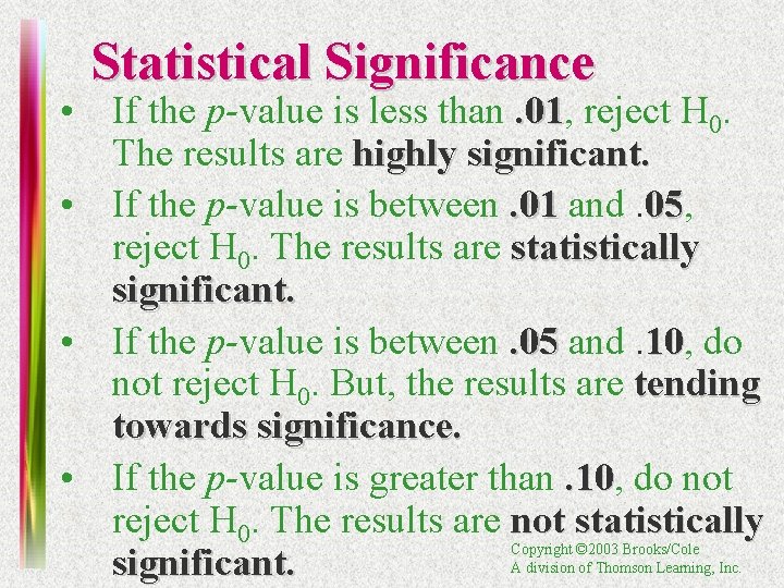
Statistical Significance • If the p-value is less than. 01, . 01 reject H 0. The results are highly significant. • If the p-value is between. 01 and. 05, 05 reject H 0. The results are statistically significant. • If the p-value is between. 05 and. 10, 10 do not reject H 0. But, the results are tending towards significance. • If the p-value is greater than. 10, . 10 do not reject H 0. The results are not statistically significant. Copyright © 2003 Brooks/Cole A division of Thomson Learning, Inc.
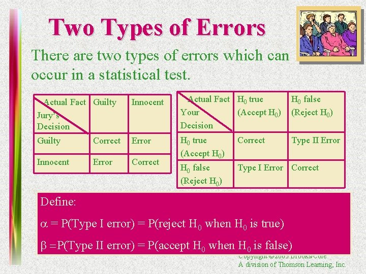
Two Types of Errors There are two types of errors which can occur in a statistical test. Actual Fact Guilty Jury’s Decision Innocent Actual Fact H 0 true Your (Accept H 0) Decision H 0 false (Reject H 0) Guilty Correct Error Correct Type II Error Innocent Error Correct H 0 true (Accept H 0) H 0 false (Reject H 0) Type I Error Correct Define: a = P(Type I error) = P(reject H 0 when H 0 is true) b =P(Type II error) = P(accept H 0 when H 0 is false) Copyright © 2003 Brooks/Cole A division of Thomson Learning, Inc.
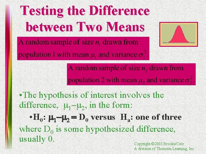
Testing the Difference between Two Means • The hypothesis of interest involves the difference, m 1 -m 2, in the form: • H 0: m 1 -m 2 = D 0 versus Ha: one of three where D 0 is some hypothesized difference, usually 0. Copyright © 2003 Brooks/Cole A division of Thomson Learning, Inc.
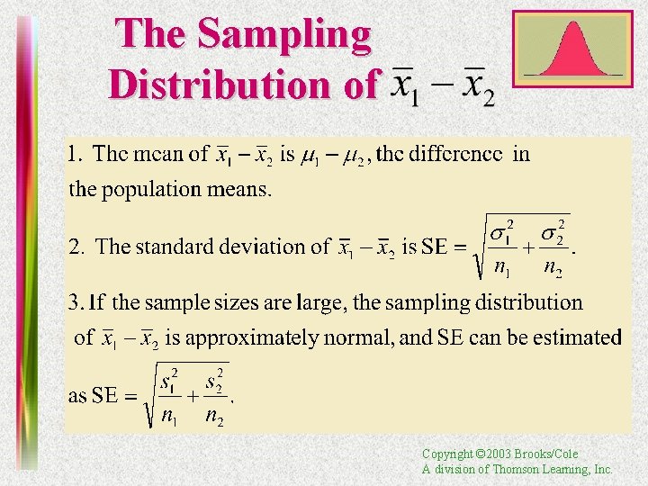
The Sampling Distribution of Copyright © 2003 Brooks/Cole A division of Thomson Learning, Inc.
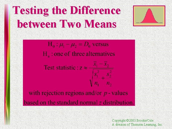
Testing the Difference between Two Means Copyright © 2003 Brooks/Cole A division of Thomson Learning, Inc.
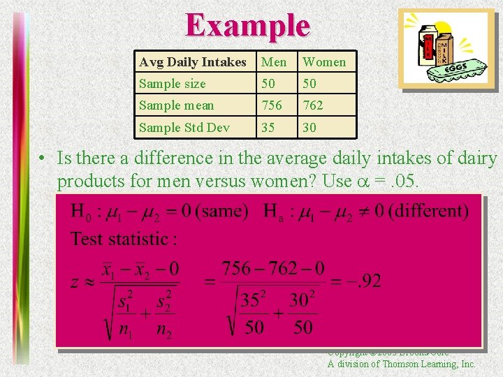
Example Avg Daily Intakes Men Women Sample size 50 50 Sample mean 756 762 Sample Std Dev 35 30 • Is there a difference in the average daily intakes of dairy products for men versus women? Use a =. 05. Copyright © 2003 Brooks/Cole A division of Thomson Learning, Inc.
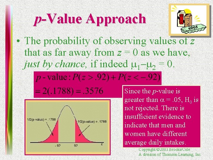
p-Value Approach • The probability of observing values of z that as far away from z = 0 as we have, just by chance, if indeed m 1 -m 2 = 0. Since the p-value is greater than a =. 05, H 0 is not rejected. There is insufficient evidence to indicate that men and women have different average daily intakes. Copyright © 2003 Brooks/Cole A division of Thomson Learning, Inc.
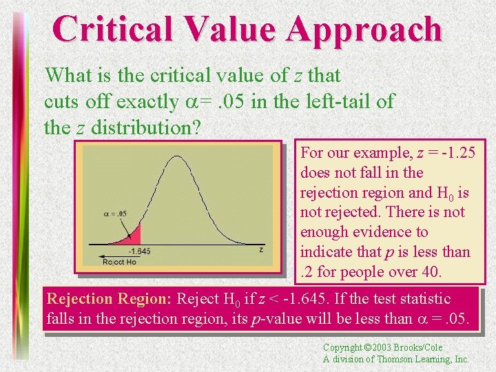
Critical Value Approach What is the critical value of z that cuts off exactly a=. 05 in the left-tail of the z distribution? For our example, z = -1. 25 does not fall in the rejection region and H 0 is not rejected. There is not enough evidence to indicate that p is less than. 2 for people over 40. Rejection Region: Reject H 0 if z < -1. 645. If the test statistic falls in the rejection region, its p-value will be less than a =. 05. Copyright © 2003 Brooks/Cole A division of Thomson Learning, Inc.
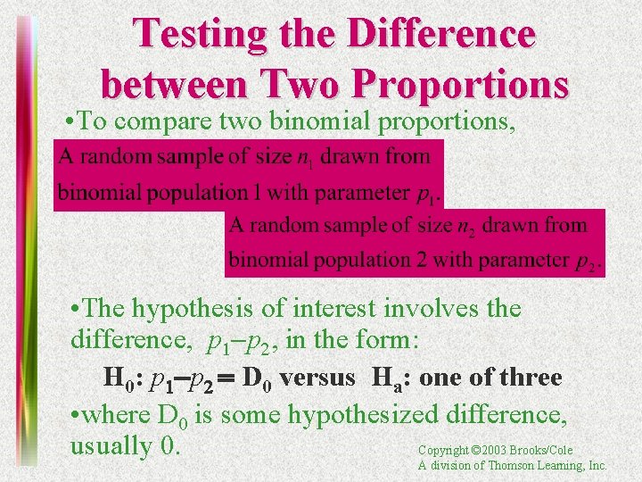
Testing the Difference between Two Proportions • To compare two binomial proportions, • The hypothesis of interest involves the difference, p 1 -p 2, in the form: H 0: p 1 -p 2 = D 0 versus Ha: one of three • where D 0 is some hypothesized difference, usually 0. Copyright © 2003 Brooks/Cole A division of Thomson Learning, Inc.
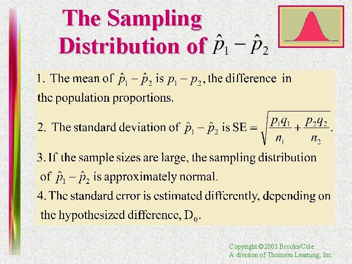
The Sampling Distribution of Copyright © 2003 Brooks/Cole A division of Thomson Learning, Inc.
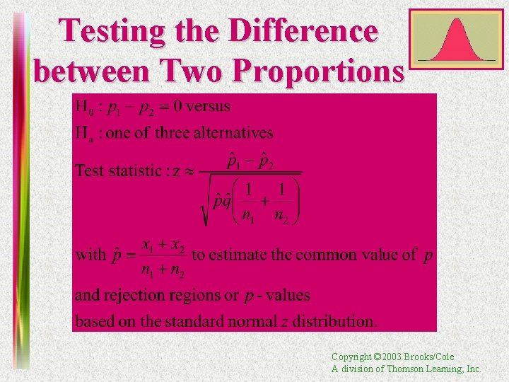
Testing the Difference between Two Proportions Copyright © 2003 Brooks/Cole A division of Thomson Learning, Inc.
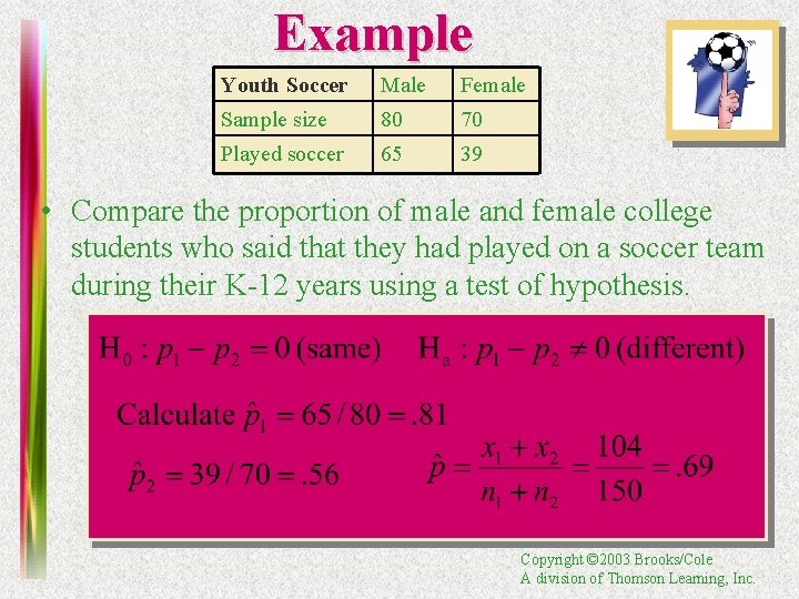
Example Youth Soccer Male Female Sample size 80 70 Played soccer 65 39 • Compare the proportion of male and female college students who said that they had played on a soccer team during their K-12 years using a test of hypothesis. Copyright © 2003 Brooks/Cole A division of Thomson Learning, Inc.
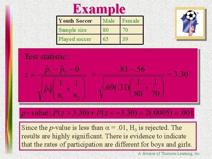
Example Youth Soccer Male Female Sample size 80 70 Played soccer 65 39 Since the p-value is less than a =. 01, H 0 is rejected. The results are highly significant. There is evidence to indicate that the rates of participation are different. Copyright for boys and girls. © 2003 Brooks/Cole A division of Thomson Learning, Inc.
- Slides: 102