Sampling Distribution of the Sample Proportion Let p

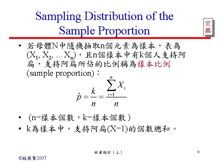
Sampling Distribution of the Sample Proportion • Let p denote the proportion of items in a population that possess a certain characteristic (unemployed, income below poverty level). • To estimate p, we take a random sample of n observation from the population and count the number X of items in the sample that possess the characteristic. • The sample proportion p^ = X/n is used to estimate the population proportion p. 社會統計(上) ©蘇國賢 2007 3
 = p • P(X=0) = (1 -p)")
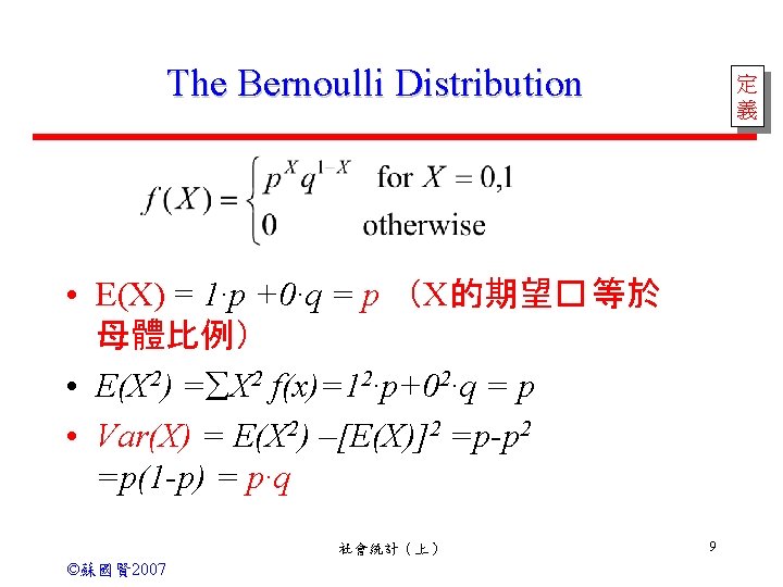
The Bernoulli Distribution 定 義 • P(X=1) = p • P(X=0) = (1 -p) • If we let q = 1 - p, then the p. f of X can be written as follows: 社會統計(上) ©蘇國賢 2007 8

Sampling Distribution of the Sample Proportion • The Normal Approximation Rule for Proportion: Let p denote the proportion of a population possessing some characteristics of interest. Take a random sample of n observations from the population. Let X denote the number of items in the sample possessing the characteristic. We estimate the population proportion p by the sample proportion p^=X/n. If np 5, and nq 5, the random variable p^ has approximately a normal distribution with: 社會統計(上) ©蘇國賢 2007 10
 ©蘇國賢 2007 11")
Sampling Distribution of the Sample Proportion • 證明 社會統計(上) ©蘇國賢 2007 11

Sampling Distribution of the Sample Proportion • 證明 assume X 1, X 2…Xn independent 社會統計(上) ©蘇國賢 2007 12

Sampling Distribution of the Sample Proportion • If the distribution of p^ is approximately normal, and 社會統計(上) ©蘇國賢 2007 13

例題 • Of your first 15 grandchildren, what is the chance there will be more than 10 boys? (assume equal probability of male/female) • “more than 10 boys” ”the proportion of boys is more than 10/15” • Use the Normal Approximation Rule: 社會統計(上) ©蘇國賢 2007 15
 we know that p^ ~N(p, pq/n) , where")
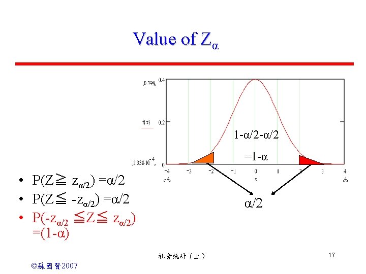
Confidence intervals for proportions (large samples) we know that p^ ~N(p, pq/n) , where q = 1 -p and np≧ 5 and nq≧ 5) 社會統計(上) ©蘇國賢 2007 16
 上面的公式必須要有母體比例p才能估計標準誤 社會統計(上) ©蘇國賢 2007 18")
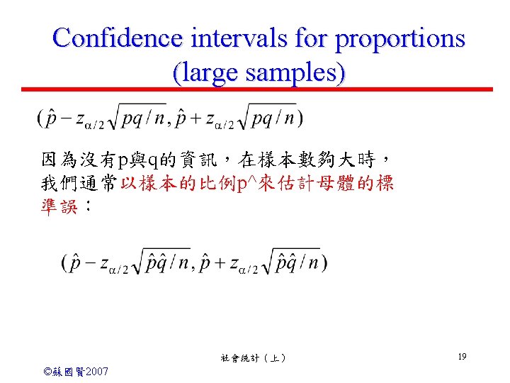
Confidence intervals for proportions (large samples) 上面的公式必須要有母體比例p才能估計標準誤 社會統計(上) ©蘇國賢 2007 18

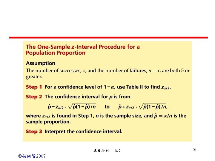
Confidence interval for the population proportion p 定 義 Let p denote the population proportion. Suppose we take a large random sample of n observations and obtain the sample proportion p^. A confidence interval for the population proportion having level of confidence 100(1 -α)% is given by 社會統計(上) ©蘇國賢 2007 20
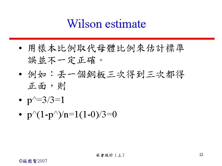

Wilson estimate We must know the s. d. of the population to get a CI for p. • Unfortunately, modern computer studies reveal the confidence intervals based on this approach can be quite inaccurate, even for large samples. -- When the sample is not a SRS. -- When the sample size is small 社會統計(上) ©蘇國賢 2007 23

Wilson estimate • The Wilson estimate ~ Add 2 successes and 2 failures (so that the sample proportion is slightly moved away from 0 and 1. ) -- Because this estimate was first suggested by Edwin Bidwell Wilson in 1927, we call it the Wilson estimate. 社會統計(上) ©蘇國賢 2007 24

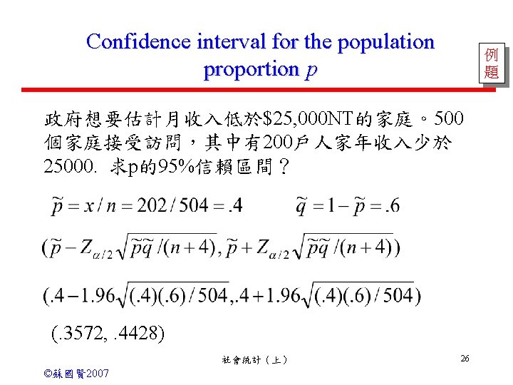
Wilson estimate 的抽樣分配趨近於平均數為p、標準差為 的常態分配。 • An approximate level C confidence interval for p is • • The margin of error is 社會統計(上) ©蘇國賢 2007 25


One-sided confidence intervals for the population proportion Suppose that we take a random sample of n observations from some population having unknown proportion p. Suppose we wish to find the lower confidence limit LCL such that the probability is (1 ) that p exceeds LCL. The one-sided interval (LCL, 1. 00) is a left-sided confidence interval. The LCL is given by: 社會統計(上) ©蘇國賢 2007 28

One-sided confidence intervals for the population proportion Construct a right-sided 95% CI for the proportion of defective items produced by a machine if 16 items are found to be defective in a random sample of 100 items. The 95% right-sided CI for p is (0, . 2306) This mean that we can be 95% confident that the population proportion is less than. 2306 29 社會統計(上) ©蘇國賢 2007

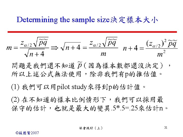
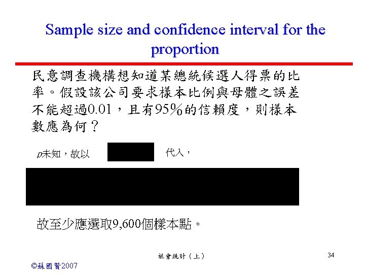
Determining the sample size決定樣本大小 Margin of Error Suppose that we take a random sample from some population. Then a 100(1 - )% confidence interval for the population proportion extends at most a distance m on each side of the sample proportion if the number of observations is ? 社會統計(上) ©蘇國賢 2007 30
:如果母體的 比例為p, 且np 5 and nq 5, 則樣本比")
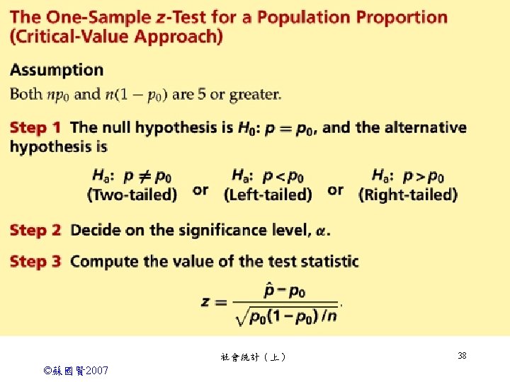
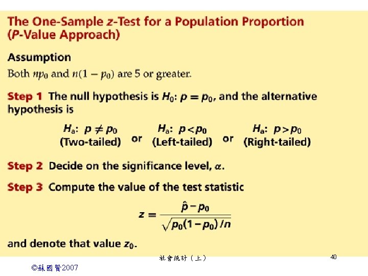
Tests of the population proportion 樣本比例的抽樣分配 f(p^):如果母體的 比例為p, 且np 5 and nq 5, 則樣本比 例p^為一常態分配~N(p, pq/n) The Normal Approximation Rule for Proportion: If np 5, and nq 5, the random variable p^ has approximately a normal distribution with: 社會統計(上) ©蘇國賢 2007 35

Sampling Distribution of the Sample Proportion • If the distribution of p^ is approximately normal, then random variable 社會統計(上) ©蘇國賢 2007 36

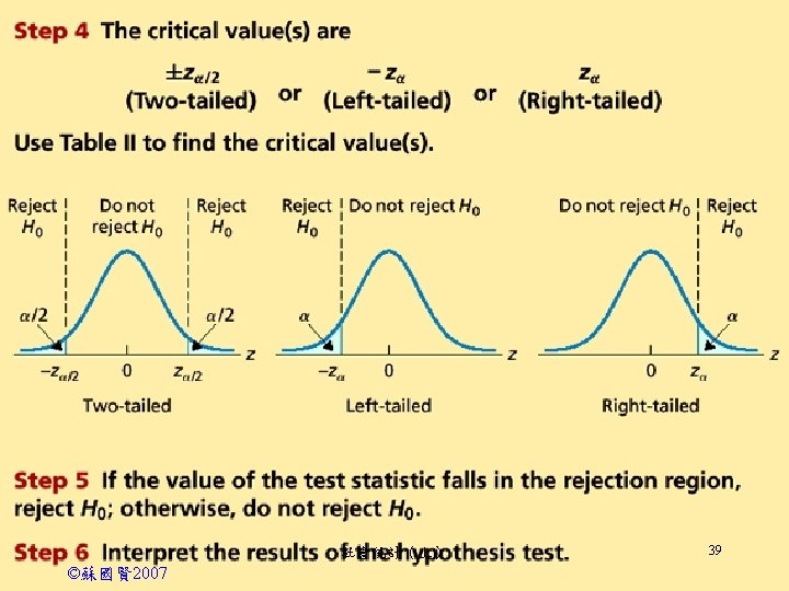
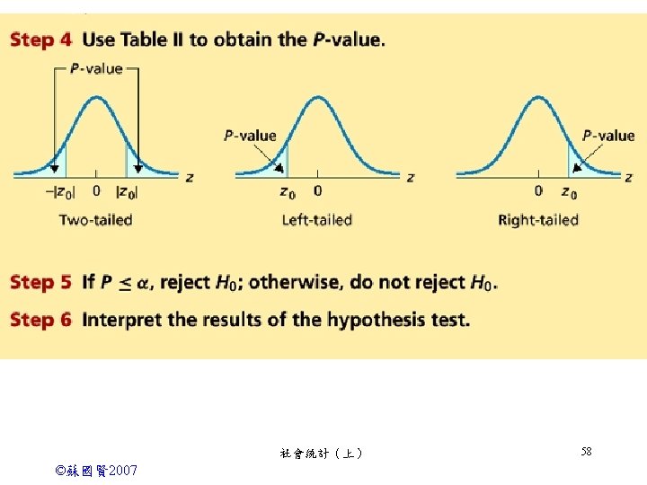
Tests of the population proportion 設np 5 and nq 5 檢證下列假說: H 0: p = p 0 or H 0: p p 0 H 1: p < p 0 如果H 0為真,則樣本比率~N(p 0, p 0 q 0/n) 假設為真時的母體比例 Reject H 0 if Z < -z or p^ < p^* (critical value approach) 社會統計(上) ©蘇國賢 2007 37
 社會統計(上) ©蘇國賢 2007 41")
Page 614, Procedure 12. 2 B (cont. ) 社會統計(上) ©蘇國賢 2007 41
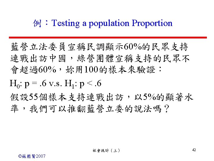

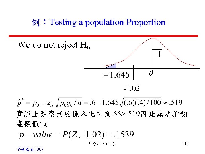
例:Testing a population Proportion Solution: If H 0 is true, then p^ has a normal distribution with mean p =. 6 and variance pq/n = (. 6)(. 4)/100 =. 0024 If we use a one-tailed test at the 5% level of significance, the critical region consists of all values of Z less than –z = -z. 05 = -1. 645 從樣本中得知p^=x/n = 55/100 =. 55 社會統計(上) ©蘇國賢 2007 43

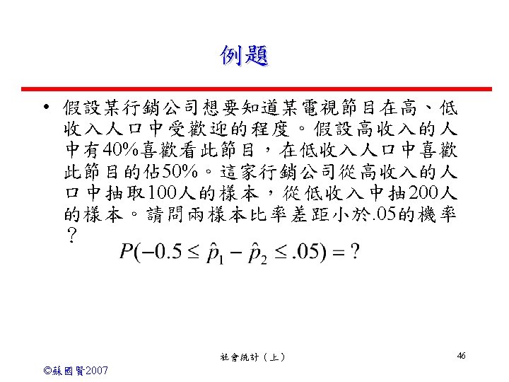
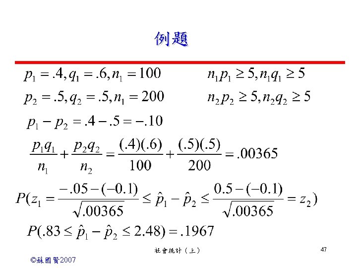
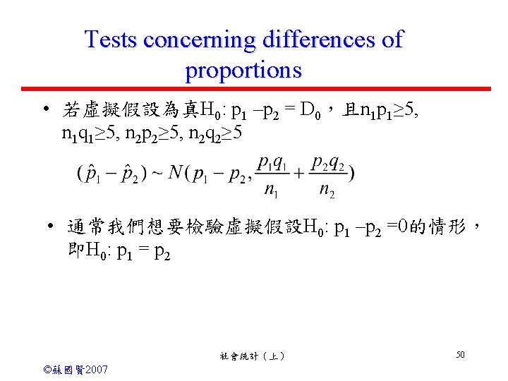
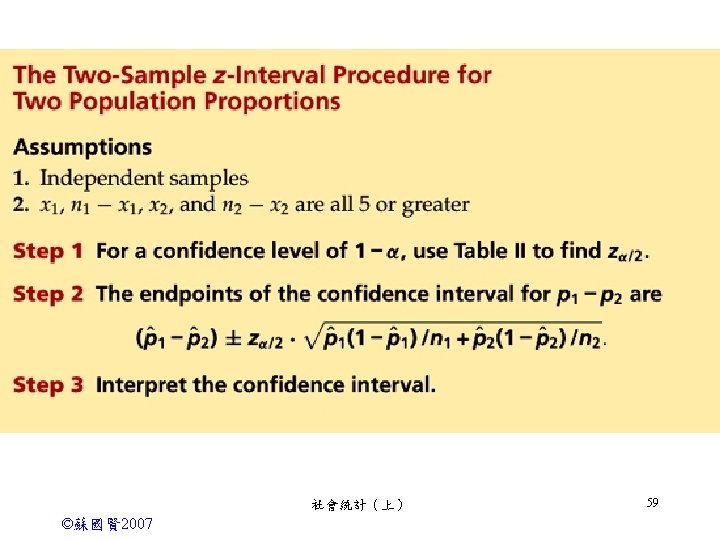
Sampling distribution of the difference between sample proportions • Suppose we take independent sample of size n 1 and n 2 from two population. Let p 1 and p 2 be the proportion of items in each population that possess a certain characteristics, and let q 1=(1 p 1), q 2=(1 -p 2). If n 1 p 1>5, n 1 q 1>5, n 2 p 2>5, n 2 q 2>5, then the random variable (p 1^-p 2^) is approximately normally distributed with 社會統計(上) ©蘇國賢 2007 45

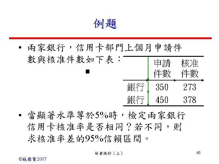
Confidence intervals for the difference of Two population proportion Let p 1 denote the observed proportion of successes in a random sample of n 1 observation from a population with proportion p 1 successes, and let p 2 denote the observed proportion of successes in an independent random sample of n 2 observations from a population with proportion p 2 successes. A 100(1 - α) % confidence interval for (p 1 – p 2) is given by the interval This result holds provided n 1 p 1≧ 5 n 1 q 1 ≧ 5 n 2 p 2≧ 5 and n 2 q 2 ≧ 5 社會統計(上) ©蘇國賢 2007 48
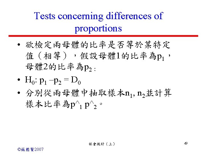

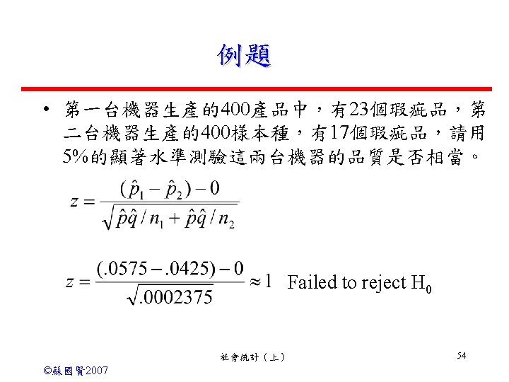
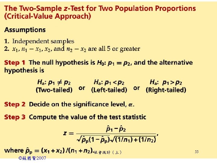
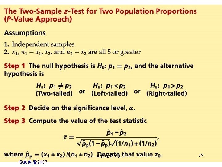
Tests concerning differences of proportions 檢定 H 0: p 1 – p 2 =0 v. s. H 1: p 1 – p 2 ≠ 0 社會統計(上) ©蘇國賢 2007 52

- Slides: 61