Salinity is the total amount of solid materials

. The ratio of the more abundant")


 method (precision ± 0. 02, prior to 1960) • time")
 ΔT ± 0.")

 • Determine the depth a water mass settles in equilibrium.")

 on temperature")
 accuracy: ± 0. 5 kg/m 3 where ρ0=1027 kg/m 3, T")
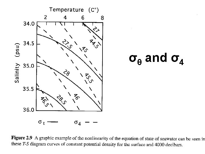
 and σt σt as a function of T and S")
 Specific volume anomaly: δ=")
=0. 97266 x")


- Slides: 22
Salinity is the total amount of solid materials in grams dissolved in one kilogram of sea water On average, there is around 35 gram salt in a kilogram of sea water, 35 g/kg, written as S=35‰ or S=35 ppt, read as “thirty-five parts per thousand” Globally, S can go from near 0 (coast) to about 40 ppt (Red Sea), BUT 90% is between 34 -35 ppt The most abundant ions in sea water: chlorine Cl- 55. 0% sodium Na+ 30. 6% sulphate SO 4++ 7. 7% magnesium Mg++ 3. 7% potassium K+ 1. 1%
Basic properties of salt in sea water 1). The ratio of the more abundant components remain almost constant. (ocean is very well mixed globally over geological time) 2). There are significant differences in total concentration of the dissolved salts from place to place and at different depths. (Oceanic processes, such as local evaporation and precipitation, continually concentrate and dilute salt in sea water in specific localities) 3). The presence of salts influences most physical properties of sea water (density, compressibility, freezing point). 4). The conductivity of the sea water is partly determined by the amount of salt it contains.
Salinity measurement Total resolved material is hard to measure routinely in seawater (e. g. , evaporation of sea-water sample to dryness) In practice, some properties of sea water are used to determine salinity. Method #1: Salinity is determined by measurements of a substitution quantity since it is contributed by its components in a fixed ratio. Method #2: Salinity is inferred from measurements of sea water’s electrical conductivity.
Absolute salinity SA Salinity can be determined through its most important component, chloride ion (plus the chlorine equivalent of the bromine and iodine), called as chlorinity (in 1902). Chlorinity is measured using titration method The relationship between salinity and chloride is based on laboratory measurements of sea water samples from all regions of the world ocean and was given in 1969 by UNESCO as SA (‰) = 1. 80655×Chlorinity (‰) SA is called as “Absolute Salinity”, unit: ppt
Practical salinity S • The practical salinity, symbol S, of a sample of sea water, is defined in terms of the ratio K of the electrical conductivity of a sea water sample of 15°C and the pressure of one standard atmosphere, to that of a potassium chloride (KCl) solution, in which the mass fraction of KCl is 0. 0324356, at the same temperature and pressure. The K value exactly equal to one corresponds, by definition, to a practical salinity equal to 35. • The corresponding formula is: S = 0. 0080 - 0. 1692 K 1/2 + 25. 3853 K + 14. 0941 K 3/2 - 7. 0261 K 2 + 2. 7081 K 5/2 • Note that in this definition, S is a ratio and is non-dimensional, but salinity of 35‰ corresponds to a value of 35 in the practical salinity. • S is sometimes given the unit “psu” (practical salinity unit) in literature (probably unnecessarily)
Salinity measurement Knudsen (Titration) method (precision ± 0. 02, prior to 1960) • time consuming and not convenient on board ship • not accurate enough to identify deep ocean water mass Electrical conductivity method (precision ± 0. 003~± 0. 001) • Conductivity depends on the number of dissolved ions per volume (i. e. salinity) and the mobility of the ions (ie temperature and pressure). Its units are m. S/cm (milli. Siemens per centimetre). • Conductivity increases by the same amount with ΔS~0. 01, ΔT~ 0. 01°C, and Δz~ 20 m. • The conductivity-density relation is closer than densitychlorinity • The density and conductivity is determined by the total weight of the dissolved substance
conductivity-temperature-depth probe In situ CTD precision: ΔS~± 0. 005 (0. 001) ΔT ± 0. 005 K (0. 001 K) Δz~± 0. 15%×z (5%) The vertical resolution is high CTD sensors should be calibrated (with bottle samples before 1990 s)
Modern subsurface floats remain at depth for a period of time, come to the surface briefly to transmit their data to a satellite and return to their allocated depth. These floats can therefore be programmed for any depth and can also obtain temperature and salinity (CTD) data during their ascent. The most comprehensive array of such floats, known as Argo, began in the year 2000. Argo floats measure the temperature and salinity of the upper 2000 m of the ocean. This will allow continuous monitoring of the When the Argo programme is fully operational it will climate state of the ocean, have 3, 000 floats in the world ocean at any one time. with all data being relayed and made publicly available within hours after collection. Subsurface drifters
Density (ρ, kg/m 3) • Determine the depth a water mass settles in equilibrium. • Determine the large scale circulation. • ρ changes in the ocean is small. 1020 -1070 kg/m 3 (depth 0~10, 000 m) • ρ increases with p (the greatest effect) ignoring p effect: ρ~1020. 0 -1030. 0 kg/m 3 1027. 7 -1027. 9 kg/m 3 for 50% of ocean • ρ increases with S. ρ decreases with T most of the time. • ρ is usually not directly measured but determined from T, S, and p
Density anomaly σ Since the first two digits of ρ never change, a new quantity is defined as σs, t, p = ρ – 1000 kg/m 3 called as “in-situ density anomaly”. (ρoo=1000 kg/m 3 is for freshwater at 4 o. C) Atmospheric-pressure density anomaly (Sigma-tee) σt = σs, t, 0= ρs, t, 0 – 1000 kg/m (note: s and t are in situ at the depth of measurement)
The Equation of the State The dependence of density ρ (or σ) on temperature T, salinity S and pressure p is the Equation of State of Sea Water. Bulk modulus K=1/β, β=compressibility. , C speed of the sound in sea water. ρ=ρ(T, S, p) is determined by laboratory experiments. International Equation of State (1980) is the most widely used density formula now. • This equation uses T in °C, S from the Practical Salinity Scale and p in dbar (1 dbar = 104 Pascal = 104 N m-2) and gives ρ in kg m 3. • Range: -2 o. C≤ T ≤ 40 o. C, 0 ≤ S ≤ 40, 0 ≤ p ≤ 105 k. Pa (depth, 0 to 10, 000 m) • Accuracy: 5 x 10 -6 (relative to pure water, σt: ± 0. 005) • Polynomial expressions of ρ(S, t, 0) (15 terms) and K(S, t, p) (27 terms) get accuracy of 9 x 10 -6.
Simple formula: (1) accuracy: ± 0. 5 kg/m 3 where ρ0=1027 kg/m 3, T 0=10 o. C, S 0=35 psu, a=-0. 15 kg/m 3 o. C, b=0. 78 kg/m 3, k=4. 5 x 10 -3 /dbar (2) where For 30≤S≤ 40, -2≤T≤ 30, p≤ 6 km, good to 0. 16 kg/m 3 For 0 ≤S≤ 40, good to 0. 3 kg/m 3
Relation between (T, S) and σt σt as a function of T and S • The relation is more nonlinear with respect to T • ρ change is more uniform with S • ρ is more sensitive to S than T near freezing point • ρmax meets the freezing point at S =24. 7 S < 24. 7: after passing ρmax surface water becomes lighter and eventually freezes over if cooled further. The deep basins are filled with water of maximum density The temperature of density maximum is the red line and the freezing point is the light blue line S > 24. 7: Convection always reaches the entire water body. Cooling is slowed down because a large amount of heat is stored in the water body
Specific volume and anomaly Specific volume: α=1/ρ (unit m 3/kg) Specific volume anomaly: δ= αs, t, p – α 35, 0, p (usually positive) • δ = δs + δt + δs, p + δt, p + δs, t, p • In practice, δs, t, p is always small (ignored) • δs, p and δt, p are smaller than the first three terms (5 to 15 x 10 -8 m 3/kg per 1000 m) Thermosteric anomaly: ΔS, T = δs + δt + δs, t (50 -100 x 10 -8 m 3/kg or 50 -100 centiliter per ton, c. L/t)
Converting formula for ΔS, T and σt : Since α(35, 0, 0)=0. 97266 x 10 -3 m 3/kg, , m 3/kg For 23 ≤ σt ≤ 28, , accurate to 0. 1 accurate to 1 in c. L/ton For most part of the ocean, 25. 5 ≤σt≤ 28. 5. Correspondingly, 250 c. L/ton ≥ ΔS, T ≥ -50 c. L/ton
Potential temperature In situ temperature is not a conservative property in the ocean. Changes in pressure do work on a fluid parcel and changes its internal energy (or temperature) compression => warming expansion => cooling The change of temperature due to pressure work can be accounted for Potential Temperature: The temperature a parcel would have if moved adiabatically (i. e. , without exchange of heat with surroundings) to a reference pressure. • If a water-parcel of properties (So, to, po) is moved adiabatically (also without change of salinity) to reference pressure pr, its temperature will be where Γ Adiabatic lapse rate: vertical temperature gradient for fluid with constant θ αT is thermal expansion coefficient • When pr=0, θ=θ(So, to, po, 0)=θ(So, to, po) is potential temperature. At the surface, θ=T. Below surface, θ<T. Potential density: σθ=ρS, θ, 0 – 1000 T is absolute temperature (o. K)
A proximate formula: t in o. C, S in psu, p in “dynamic km” For 30≤S≤ 40, -2≤T≤ 30, p≤ 6 km, θ-T good to about 6% (except for some shallow values with tiny θ-T) In general, difference between θ and T is small θ≈T-0. 5 o. C for 5 km
An example of vertical profiles of temperature, salinity and density
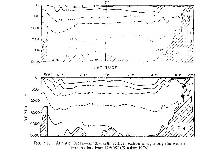
θ and σθ in deep ocean Note that temperature increases in very deep ocean due to high co mpressibility
Definitions in-situ density anomaly: σs, t, p = ρ – 1000 kg/m 3 Atmospheric-pressure density anomaly : σt = σs, t, 0= ρs, t, 0 – 1000 kg/m 3 Specific volume anomaly: δ= αs, t, p – α 35, 0, p δ = δs + δt + δs, p + δt, p + δs, t, p Thermosteric anomaly: Δs, t = δs + δt + δs, t Potential Temperature: Potential density: σθ=ρs, θ, 0 – 1000