Salient Object Detection by Composition Jie Feng 1

Salient Object Detection by Composition Jie Feng 1, Yichen Wei 2, Litian Tao 3, Chao Zhang 1, Jian Sun 2 1 Key Laboratory of Machine Perception, Peking University 2 Microsoft Research Asia 3 Microsoft Search Technology Center Asia
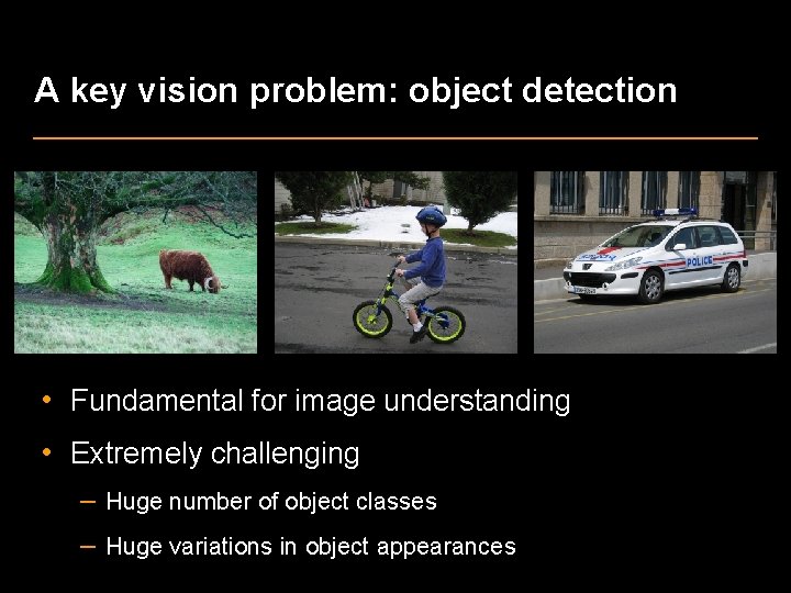
A key vision problem: object detection • Fundamental for image understanding • Extremely challenging – Huge number of object classes – Huge variations in object appearances
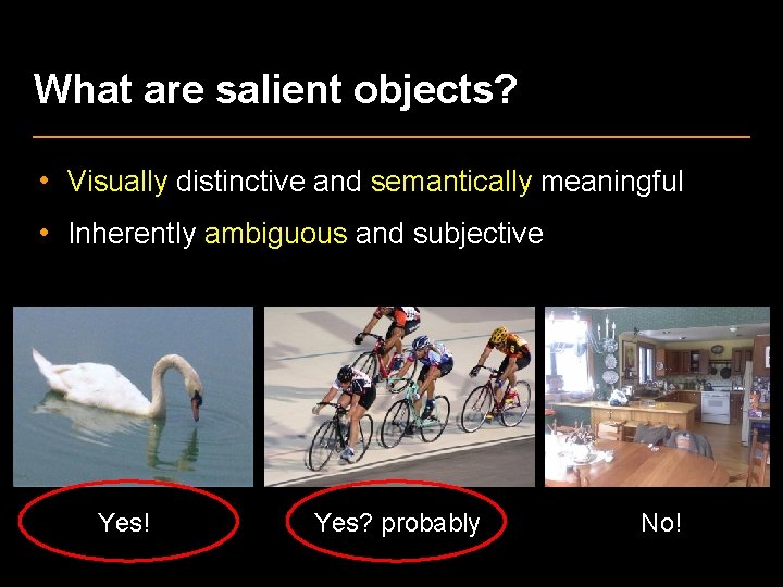
What are salient objects? • Visually distinctive and semantically meaningful • Inherently ambiguous and subjective Yes! Yes? probably No!
Why detect salient objects? • Relatively easy: large and distinct • Semantically important 1. Image summarization, cropping… 2. Object level matching, retrieval… 3. A generic object detector for later recognition – avoid running thousands of different detectors – a scalable system for image understanding
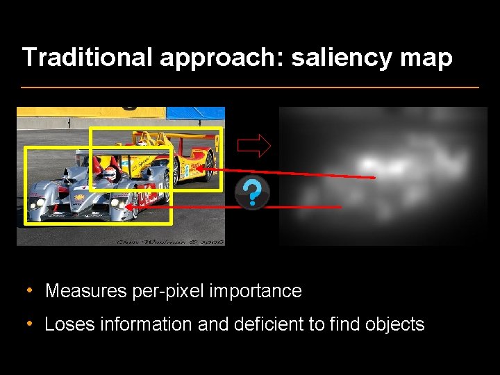
Traditional approach: saliency map • Measures per-pixel importance • Loses information and deficient to find objects

sliding window object detection • • • Face, human… Car, bus… Horse, dog… Table, couch… … • Slide different size windows over all positions • Evaluate a quality function, e. g. , a car classifier • Output windows those are locally optimum
Salient object detection by composition • A ‘composition’ based window saliency measure – intuitive and generalizes to different objects • A sliding window based generic object detector – fast and practical: 1 -2 seconds per image – a few dozens/hundreds output windows • Effective pre-processing for later recognition tasks
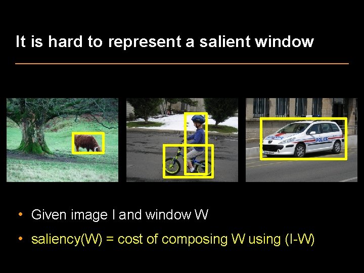
It is hard to represent a salient window • Given image I and window W • saliency(W) = cost of composing W using (I-W)
Benefits of ‘composition’ definition •
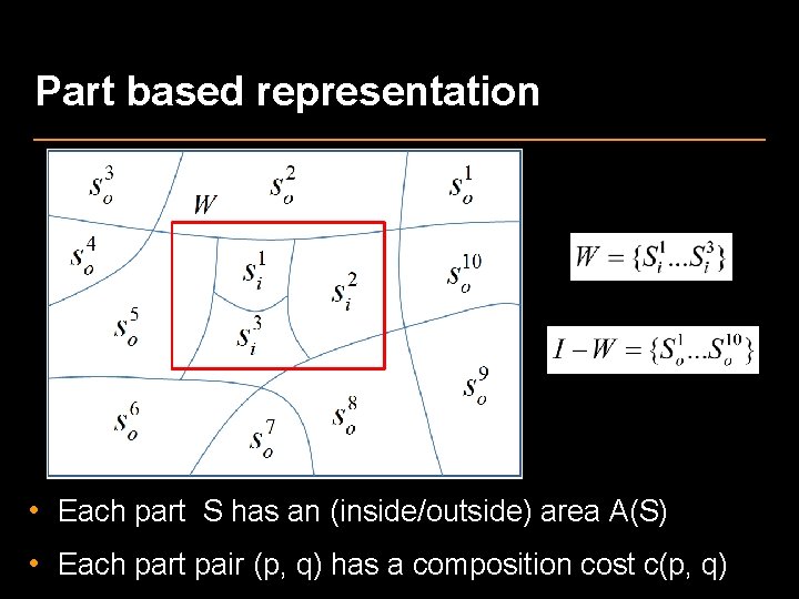
Part based representation • Each part S has an (inside/outside) area A(S) • Each part pair (p, q) has a composition cost c(p, q)
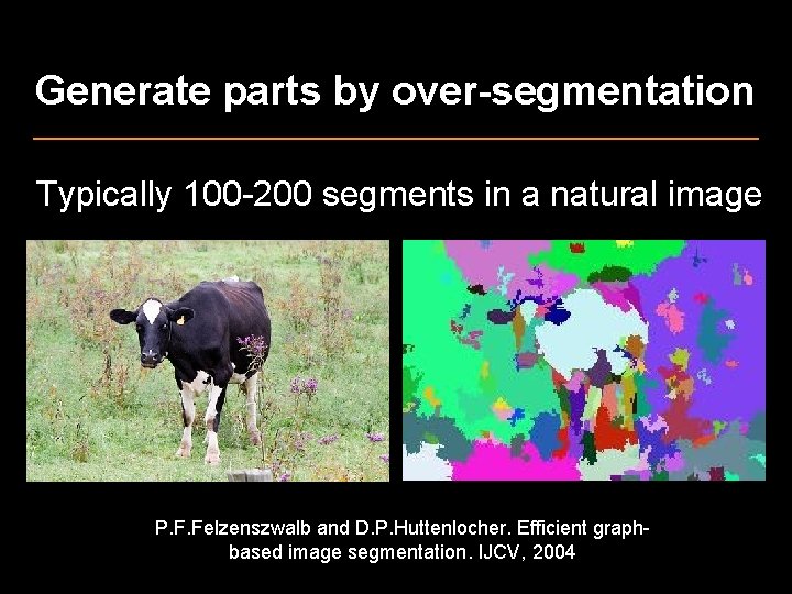
Generate parts by over-segmentation Typically 100 -200 segments in a natural image P. F. Felzenszwalb and D. P. Huttenlocher. Efficient graphbased image segmentation. IJCV, 2004
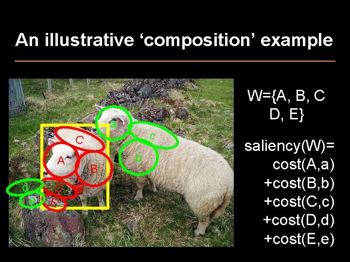
An illustrative ‘composition’ example W={A, B, C D, E} a c C A d e D E B b saliency(W)= cost(A, a) +cost(B, b) +cost(C, c) +cost(D, d) +cost(E, e)
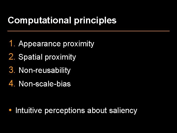
Computational principles 1. Appearance proximity 2. Spatial proximity 3. Non-reusability 4. Non-scale-bias • Intuitive perceptions about saliency
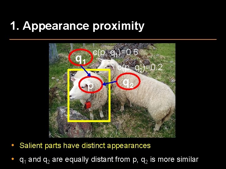
1. Appearance proximity q 1 c(p, q 1)=0. 6 c(p, q 2)=0. 2 p q 2 • Salient parts have distinct appearances • q 1 and q 2 are equally distant from p, q 2 is more similar
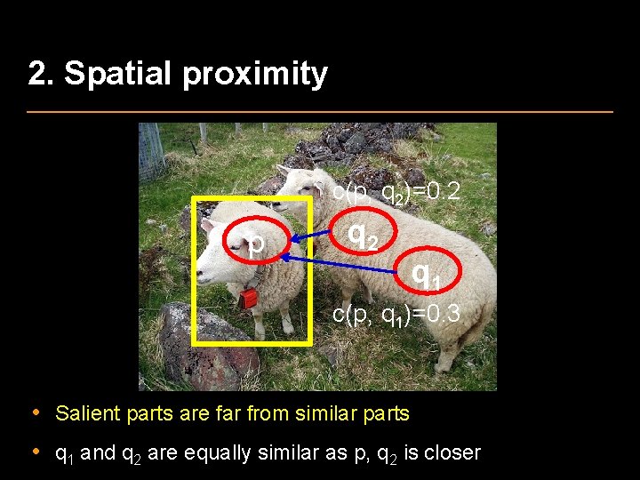
2. Spatial proximity c(p, q 2)=0. 2 p q 2 q 1 c(p, q 1)=0. 3 • Salient parts are far from similar parts • q 1 and q 2 are equally similar as p, q 2 is closer
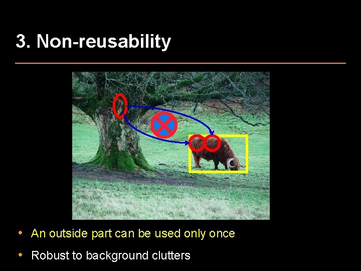
3. Non-reusability • An outside part can be used only once • Robust to background clutters
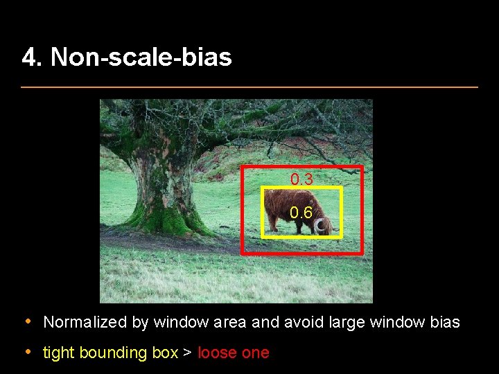
4. Non-scale-bias 0. 3 0. 6 • Normalized by window area and avoid large window bias • tight bounding box > loose one
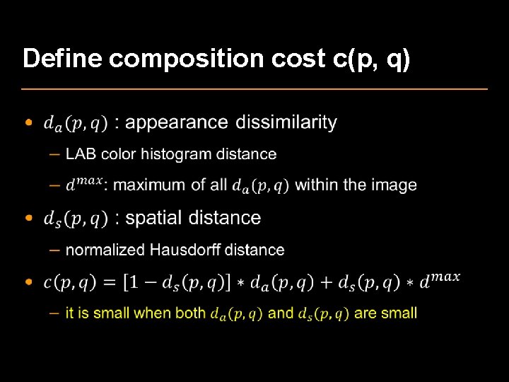
Define composition cost c(p, q) •
Part based composition • Finding outside parts with the same area of inside parts and smallest composition cost • Need to find which outside part to compose which inside part with how much area • Formulated as an Earth Mover’s Distance (EMD) – optimal solution has polynomial (cubic) complexity • A greedy optimization – pre-computation + incremental sliding window update
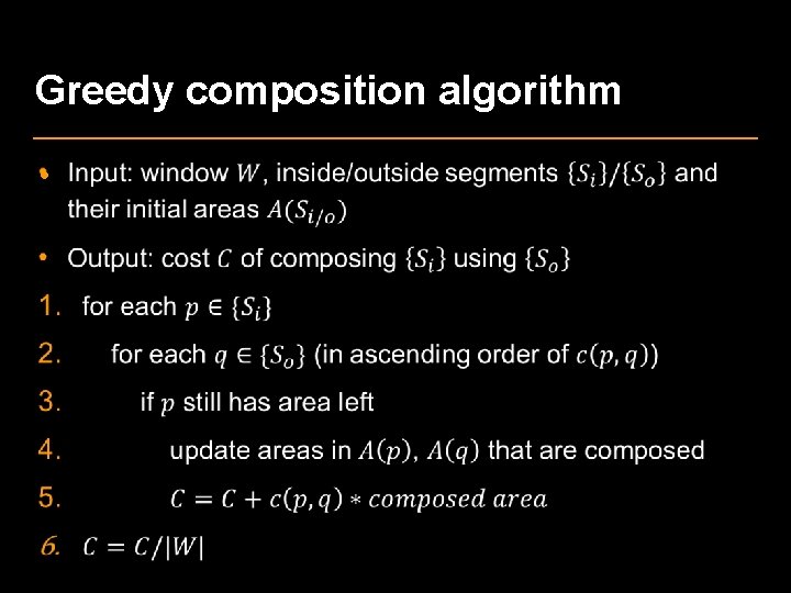
Greedy composition algorithm •
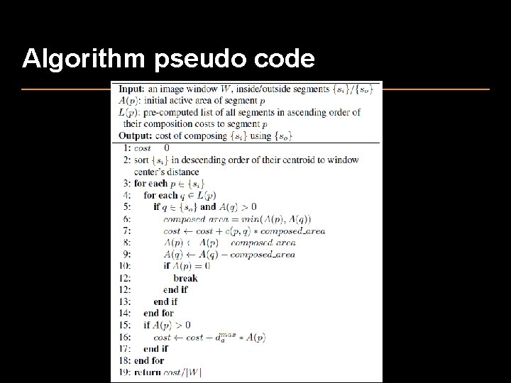
Algorithm pseudo code
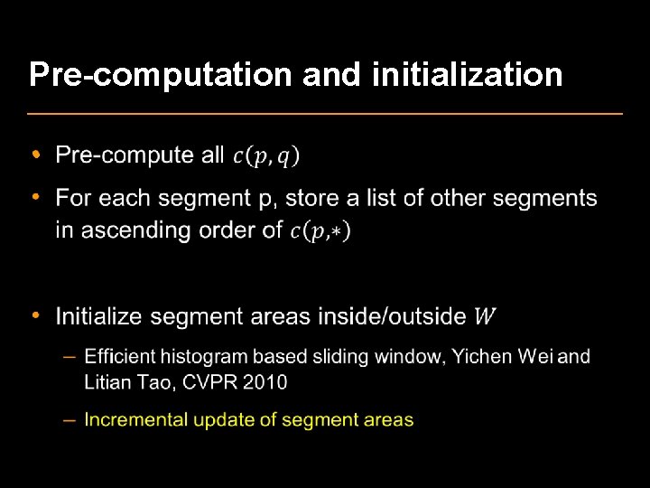
Pre-computation and initialization •
More implementation details • 6 window sizes: 2% to 50% of image area • 7 aspect ratios: 1: 2 to 2: 1 • 100 -200 segments • 1 -2 seconds for 300 by 300 image • Find local optimal windows by non-maximum suppression
Evaluation on PASCAL VOC 07 • it’s for object detection – 20 object classes – Large object and background variation – Challenging for traditional saliency methods • not totally suitable for salient object detection – Not all labeled objects are salient: small, occluded, repetitive – Not all salient objects are labeled: only 20 classes • but still the best database we have
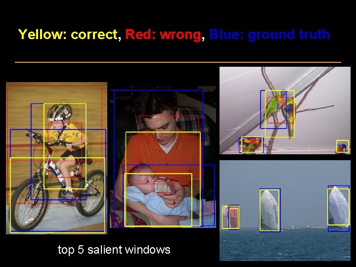
Yellow: correct, Red: wrong, Blue: ground truth top 5 salient windows

Yellow: correct, Red: wrong, Blue: ground truth
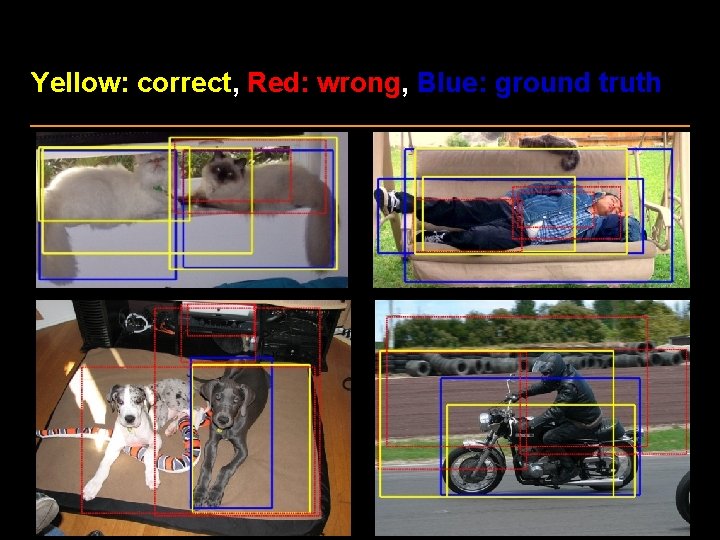
Yellow: correct, Red: wrong, Blue: ground truth
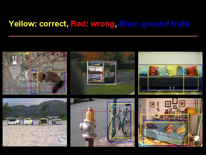
Yellow: correct, Red: wrong, Blue: ground truth
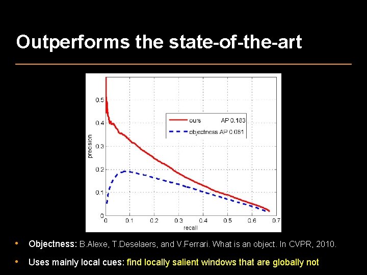
Outperforms the state-of-the-art • Objectness: B. Alexe, T. Deselaers, and V. Ferrari. What is an object. In CVPR, 2010. • Uses mainly local cues: find locally salient windows that are globally not
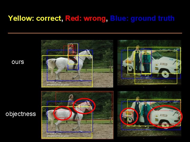
Yellow: correct, Red: wrong, Blue: ground truth ours objectness
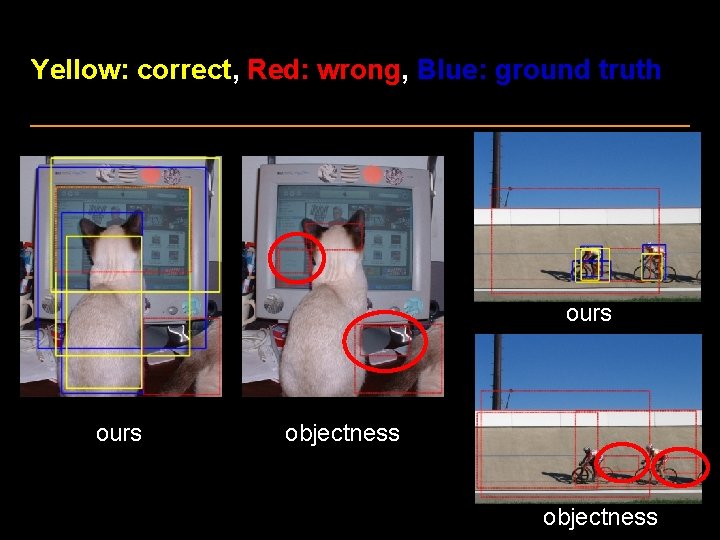
Yellow: correct, Red: wrong, Blue: ground truth ours objectness

Failure cases: too complex
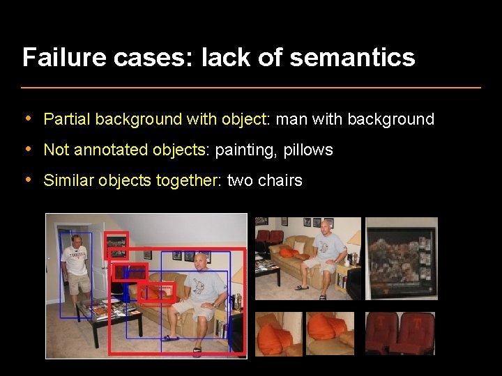
Failure cases: lack of semantics • Partial background with object: man with background • Not annotated objects: painting, pillows • Similar objects together: two chairs
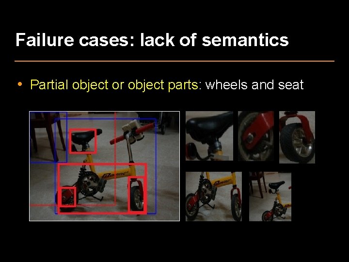
Failure cases: lack of semantics • Partial object or object parts: wheels and seat
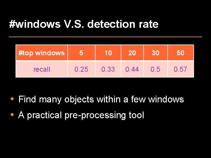
#windows V. S. detection rate #top windows 5 10 20 30 50 recall 0. 25 0. 33 0. 44 0. 57 • Find many objects within a few windows • A practical pre-processing tool

Evaluation on MSRA database • Less challenging: only a single large object – T. Liu, J. Sun, N. Zheng, X. Tang, and H. Shum. Learning to detect a salient object. In CVPR, 2007 • Use the most salient window of our approach in evaluation – pixel level precision/recall is comparable with previous methods • Our approach is principled for multi-object detection – benefits less from the database’s simplicity than previous methods
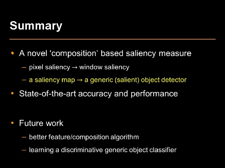
Summary •
- Slides: 37