Salahaddin UniversityErbil College of Science Physics Department Course

Salahaddin University-Erbil College of Science Physics Department Course Book Statistical Mechanics Postgraduate Students / First Course

Statistical Mechanics Fundaments of statistical physics Statistics is the study of how to collect, organize, analyze, and interpret numerical information from data. Descriptive statistics involves methods of organizing, picturing and summarizing information from data.

1. 2. 3. 4. Microstate Macrostate Partition Function Derivation of Thermodynamic laws by Statistical Mechanics 5. The idea of interaction (a) particle (system) - external environment (b) Particle (within a system of many particles) 6. Entropy: Disorder Number 7. Equipartition Theorem: the energies are distributed equally in different degrees of freedom. 8. Temperature 9. Distributions: Maxwell-Boltzmann, Fermi-Dirac, Bose. Einstein.

Why do we study Statistical Mechanics? • We apply statistical mechanics to solve for real systems (a system for many particles). • For example in an ideal gas, we assume that the molecules are non-interacting, i. e. they do not affect each other's energy levels. Each particle contains certain energy. At T> 0, the system possesses a total energy. So, how is E distributed among the particles? • Another question would be how the particles are distributed over the energy levels. We apply statistical mechanics to provide the answer and thermodynamics demands that the entropy be maximum at equilibrium. • Thermodynamics is concerned about heat and the direction of heat flow, whereas statistical mechanics gives a microscopic perspective of heat in terms of the structure of matter and provides a way of evaluating thermal properties of matter, for e. g. , heat capacity.

Variance The Variance is defined as: The average of the squared differences from the Mean Var. = σ2 And the standard deviation is the square root of the Variance • To get the standard deviation we take the square root of the variance.
 is half of the square root of")
Half Factorial The factorial of half (½) is half of the square root of π = (½)√π, and so some "half-integer" factorials are: n n! (½)√π (3/2) (3/4)√π (5/2) (15/8)√π It still follows the rule that "the factorial of any number is that number times the factorial of (1 smaller than that number)", because (3/2)! = (3/2) × (1/2)! (5/2)! = (5/2) × (3/2)! Can you figure out what (7/2)! is?

Probability distribution A distribution is the set of outcomes of a system with the probability for each outcome. It can be discrete, like a coin or die, or continuous, like a measurement of time. A (fair) die has six possible outcomes with a probability of 1/6 th for each.

A more useful measure of the scatter is given by the square root of the variance, which is usually called the standard deviation of u. The standard deviation is essentially the width of the range over which is distributed around its mean value. One can define further mean values such as ( u)n, the (nth moment of u about its mean) for integer n 2.
 After a total N steps, each")
Random Walk Problem in 1 -Dimension (binomial distribution) After a total N steps, each of length l, the particle is located at: X= ml where m is an integer lying between - N ≤ m ≤ N To calculate the probability PN(m) of finding the particle at the position x = ml after N steps. Let n 1 denote the number of steps to the right and n 2 the corresponding number of steps to the left. The total number of steps N is N = n 1 + n 2 The net displacement (measured to the right in units of a step length) is given by: m = n 1 - n 2 So m = n 1 – n 2 = n 1 – (N- n 1) = 2 n 1 – N This shows that if N is odd, the possible values of m must also be odd. Conversely, if N is even, m must also be even. The successive steps are statistically independent of each other; each step is characterized by the respective probabilities;

p = probability that the step is to the right, and q = 1 – p = probability that the step is to the left. The probability of any one given sequence of n 1 steps to the right and n 2 to the left is; pp…. . p qq…. . . q = The number of distinct possibilities (The number of sequences) is given by: N! / n 1!n 2! Hence the probability PN(n 1) of taking (in a total of N steps) n 1 steps to the right and n 2 = N – n 1 = steps to the left is given as;

Exponential distribution The Exponential distribution with parameter λ is a continuous distribution whose support is the semiinfinite interval [0, ∞). Its probability density function is given by: and it has expected value μ = λ− 1. The variance is equal to: So for an exponentially distributed random variable σ2 = μ 2.

The position of a particle is a point having the coordinates x, y, z in ordinary three dimensional space. This combination position and momentum space is called phase space, which is a six dimensional space. At any instant of time, suppose one of the particles have its position co-ordinates lying between x and x+dx, y and y+dy, z and z+dz and let its momentum coordinates lie between px and px+ dpx, py and py+ dpy, pz and pz+dpz. Thus every particle is completely specified by a point in phase space.

The volume of the cell in the phase space is dv = dxdydzdpxdpydpz According to the uncertainty principle dxdpx = dydpy = dzdpz = h Then the smallest "cell" in phase space which we can consider is constrained by the uncertainty principle to be dvminimum = h 3 =dxdpxdydpydzdpz The minimum volume of an elementary cell in phase space in Quantum Mechanical system is h 3, where h is Planck’s constant Total number of elementary cells in phase space =Total volume in phase space/Volume of one elementary cell = ∫dx∫dy∫dz ∫∫∫dpx dpy dpz / dv
 Statistics.")
Statistical distribution laws Types of statistics 1 - Classical Statistics (Maxwell – Boltzmann) Statistics. There is no restrictions on the quantity of energy, the number of molecules that are populated in any state. 2 - Quantum Statistics (Bose – Einstein And Fermi. Dirac) Statistics. Energy has been quantized • The statistical mechanics is used to determine the most probable way in which a fixed total amount of energy is distributed among the various members of an assembly of identical particles, that is, how many particles are likely to have the energy E 1, how many to have energy E 2, and so on.

• According to the modern quantum statistics, thermodynamical probability of any system for any state depends on the : what statistics do the molecules depend? • Consider three kinds of particles:

1 - Identical particles of any spin that are sufficiently widely separated to be distinguished. The molecules of a gas are particles of this kind and the Maxwell. Boltzman distribution law holds for them. 2 - Identical particles of zero or integral spin that cannot be distinguished one from another. Such particles do not obey the exclusion principle, and the Bose-Einstein distribution law holds for them. Ex. (bosons) photons or alpha particles. 3 - Identical particles of spin (1/2) that cannot be distinguished one from another. Such particles obey the exclusion principle, and the Fermi- Dirac distribution law holds for them. Ex. electrons or protons.

Basic Approach In The Three Statistics • The basic approach in three statistics is essentially the same but we get the different results due to different assumptions. The common approach is as follows: • In any dynamic isolated system, the total number of particles (N) and the total energy (E) has to remain constant. N = ∑ni = constant d. N = ∑ dni = 0 ----(1) E = ∑ Eini = constant d. E = ∑Eidni = 0 ----(2)
 with -α, eq. (2) by -β and add to eq.")
We multiply eq. (1) with -α, eq. (2) by -β and add to eq. (3) d(ln P) -α ∑ dni - β ∑ Ei dni = 0 d(ln P) - ∑ ( α + β Ei )dni = 0 ----- (4) Where and are constant quantities independent of the ni.
 • Consider a number of")
Classical statistical mechanics Maxwell – Boltzmann distribution (M-B distribution) • Consider a number of N particles of energy level 1, 2, 3, …. . , n with energy E 1, E 2, E 3, …. En. • If there are gi cells with energy Ei, the number of ways in which one particle can have the energy Ei is gi. • The total number of ways (Pi) that ni particles can have the energy Ei is (gi)ni. • Hence the number of ways in which all N particles can be distributed among the various energies is: (P 1)(P 2)(P 3)…= (g 1)n 1(g 2)n 2(g 3)n 3 ………

Example Suppose 4 particles can be distributed among 2 energy levels as; n 1=2, g 1=3, n 2= 2, g 2=2. Find the number of ways of particles distribution among: a) each level, b) the two levels, c) also find the most probable distribution. Using M. B. distribution. a) P 1 = (g 1)n 1 = 32 = 9 P 2= (g 2)n 2 = 22 = 4 b) ways. c) The most probable distribution = 6 36 = 216 ways.

Example Calculate the most probable distribution of distributing 3 objects a, b and c into two cells of two energy levels with the occupation {1, 2}. Answer: Therefore, there are three ways (3! / 1! 2! ) (1)1(1)2 = 3 | a | b c |, | b | c a |, | c | a b |. Example Calculate the number of ways of distributing 20 objects into six cells of six possible energy levels with the arrangement {1, 0, 3, 5, 10, 1). Most probable distribution: ……. (20! / 1! 3! 5! 10! 1!)(1)1(1)3…. = 931170240
, (5, 1), (4, 2), (3, 3), (2,")
The macrostates =7 which are: (6, 0), (5, 1), (4, 2), (3, 3), (2, 4), (1, 5) and (0, 6) The microstates are: For(6, 0) macrostate ways From(5, 1) macrostate ways And so on for the other macrostates.
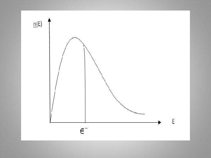
 This law is known as Maxwell-Boltzmann law of energy distribution and")
- i=0 …………………(5) This law is known as Maxwell-Boltzmann law of energy distribution and e i Boltzmann factor. This formula gives the number of particles ni that have the energy i in terms of the number of cells in phase space gi that have the energy i and the constants , .
 Where we use the definite integral Or Hence ………(10)")
By integrating equ. (9) Where we use the definite integral Or Hence ………(10)
 FMB which is proportional to the probability that")
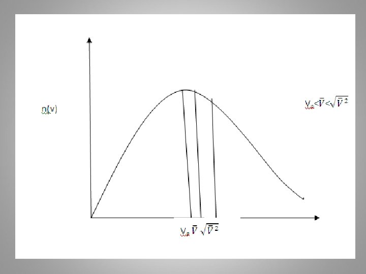
The Maxwell –Boltzmann distribution function (FMB) FMB which is proportional to the probability that a particle will be found in the state has the form, or FMB =P(V) the probability. ………(18) Where 4πv 2 dv the volume of a spherical shell of radius v and thickness dv in speed space.
 for a Maxwell- Boltzmann distribution. Solution")
2 - Find the most probable speed (vp) for a Maxwell- Boltzmann distribution. Solution The most probable speed in the M. B. distribution is that for which n(v) =4πv 2 FMB is maximum or From equation (19)

H. W • Given the distribution function: • Consider a mixture of Hydrogen and Helium at temperature T. In term of T, K, and m, find the speed at which the Maxwell distributions for these gases have the same value.
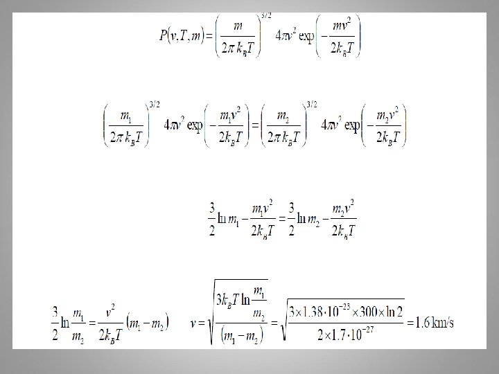

A more exact expression for the average velocity: = = Note that M is the molar mass and that the gas constant R is used in the expression. k is the Boltzmann constant. If you multiply k by Avogadro's number, you'll get R. vp= Vrms = = Make sure that you see that vrms = , not vrms =. The latter equation reduces to vrms = , which is not the case. v rms requires the mean of the squares of the velocities. Square the velocities first, then take their mean.

Dependence of Maxwell-Boltzmann speed distribution on Temperature The total area underneath the Maxwell-Boltzmann speed distributions is equal to the total number of molecules {. If the area under the two curves is equal, then the total number of molecules in each distribution are equal.

Applications of M. B distribution • The Doppler broadening of spectral lines • One of the effects which arise from the distribution of the velocities of the molecules in a hot gas at low densities is the brooding of the spectral lines which are emitted by the gas molecules. This broadening can be used as an experimental check for the validity of the Maxwell Boltzmann velocity distribution. This broadening (i. e. spread) arises from the distribution of velocities of the molecules in a gas.

The Einstein diffusion equation

The Einstein diffusion equation • bb
 The Bose-Einstein distribution describes the statistical behavior")
Quantum statistical mechanics Bose-Einstein distribution (B-E distribution) The Bose-Einstein distribution describes the statistical behavior of integer spin particles (bosons). Basic postulates In B-E statistics, the conditions are: 1 -The particles of the system are identical and indistinguishable. 2 -Any number of particles can occupy a single cell in the phase space. 3 -The size of the cell cannot be less than h 3, where h is a Plank’s constant. 4 -The number of phase space cells is comparable with the number of particles, i. e. , the occupation index f(εi) is ni/gi ≈ 1. 5 -B-E statistics is applicable to particles with integral spin. All particles which obey B. E statistics are known as Bosons.

Example: Find the distribution way for one level contains one cell non degenerate. Pi = = = There is only one way of distribution for any number of particles. =1

1+ and β= -------------23 This equation represents the most probable distribution of the particles among various energy levels for a system obeying BE statistics and is therefore, known as Bose-Einstein’s distribution law for an assembly of bosons. For photonic gas because the number of photons are not constant, so from Lagrange’s method or α =0 for photonic gas then B-E distribution for photonic gas becomes ----- 24
 The Fermi-Dirac distribution applies to fermions, particles with half -integer")
Fermi-Dirac Distribution (carriers concentration) The Fermi-Dirac distribution applies to fermions, particles with half -integer spin which must obey the Pauli exclusion principle. Basic postulates Fermi- Dirac statistics is apply to indistinguishable particles which are generated by the Pauli exclusion principle which states that no two particles can occupy the same quantum state, so the number of allowed level cannot be more than the cells number (g i) in that level (gi ≥ ni ) The F-D distribution law is the same as B-E distribution law except that now each cell (that is, Quantum state) can be occupied by at most one particle. If there are (gi) cells having the same energy ϵi and if there a number of indistinguishable particles (ni) a, b, c, there are (gi ) position (cells) for (a) leaving (gi -1) position for( b) and (gi-2) position for (c ) and gi – (ni-1) positions for the last particle. (gini) positions not occupied.

Example: Suppose in the above example there are 3 particles and 2 cells PF-D impossible for F-D distribution Ex. F. D distribution two levels, n 1=2, g 1=2, n 2=1, g 2=3. Find total distributing ways for the two levels, no transition between the levels.

To find the Fermi-Dirac distribution law Take the natural logarithm of the both sides of eq. 30 Then from Stirling's formula For maximum probability, small changes dni in any of the individual ni’s must not alter.
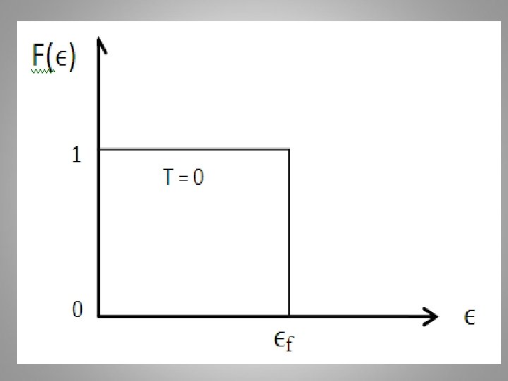

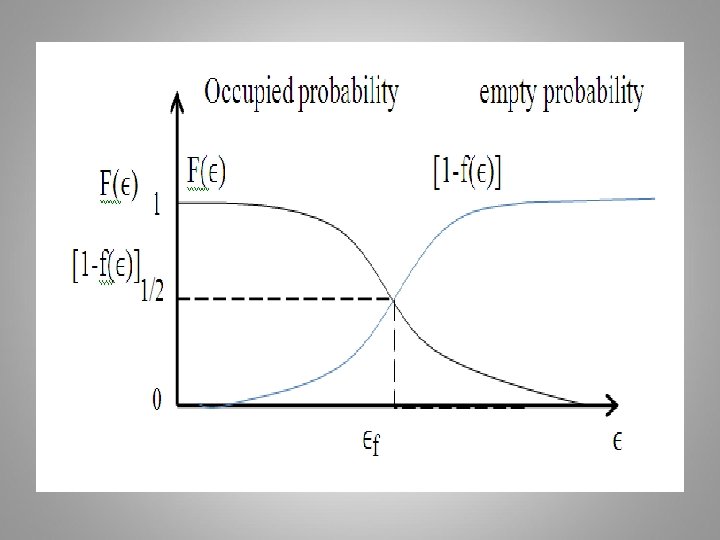
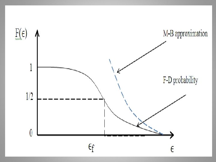
At T > 0 K If ϵ = ϵf The probability of a state occupied at ϵ = ϵf = 1/2 for all temperatures above 0 K The F-D distribution is plotted for several temperatures, assuming the Fermi energy is independent of temperature is shown below:

Example: Assume that the F-D energy level is 6. 25 e. V and that the electrons follow Fermi distribution. Calculate T at which there is a one percent probability that a state 0. 3 e. V below the Fermi energy level will not contain an electron or empty. ϵ= ϵf– 0. 30 = 6. 25 -0. 3 = 5. 95 e. V 0. 01 =1 - KT = 0. 0653 e. V 0. 0653 x 1. 6 x 10 -19 J T = 0. 0653 x 1. 6 x 10 -19 J / 1. 38 x 10 -23 = 756 K
/KT = 1/0. 5 e (E-EF)/KT = (1/")
b/ = 0. 5 1+ e (E-EF)/KT = 1/0. 5 e (E-EF)/KT = (1/ 0. 5) - 1 (E – EF)/KT = Ln (1/ 0. 5 – 1) = Ln 1 =0 E - EF= 0 x KT =0 E = EF= 5. 58 e. V

An illustrative example

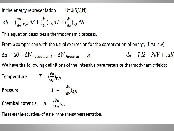
Extensive parameters of thermodynamics In the energy representation, the fundamental equation of a pure fluid is given by the relation: • U=U(S, V, N) energy representation And In the entropy is given by the relation: • S=S(U, V, N) entropy representation
- Slides: 52