S 1 Chapter 8 Discrete Random Variables www

S 1: Chapter 8 Discrete Random Variables www. drfrostmaths. com Dr J Frost (jfrost@tiffin. kingston. sch. uk) Last modified: 3 rd February 2016

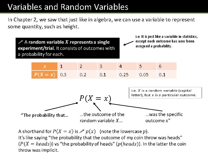
Variables and Random Variables In Chapter 2, we saw that just like in algebra, we can use a variable to represent some quantity, such as height. i. e. It is just like a variable in statistics, except each outcome has now been assigned a probability. 1 2 3 4 5 6 0. 3 0. 2 0. 1 0. 25 0. 05 0. 1 “The probability that…

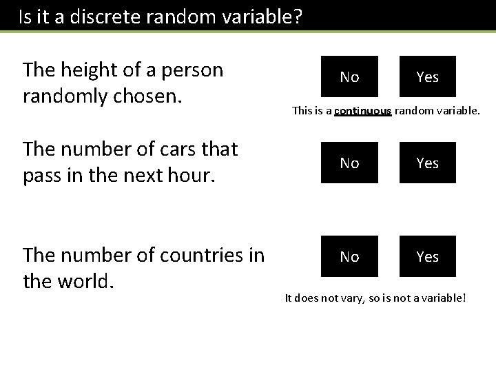
Is it a discrete random variable? The height of a person randomly chosen. The number of cars that pass in the next hour. The number of countries in the world. No Yes This is a continuous random variable. No Yes No Yes It does not vary, so is not a variable!

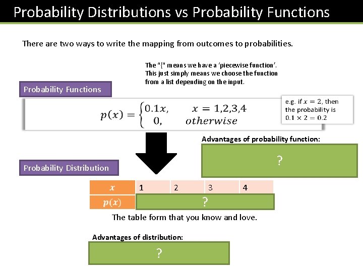
Probability Distributions vs Probability Functions There are two ways to write the mapping from outcomes to probabilities. The “{“ means we have a ‘piecewise function’. This just simply means we choose the function from a list depending on the input. Probability Functions Advantages of probability function: Can have a rule/expression based on the outcome. Particularly for continuous random variables (in S 2), it would be impossible to list the probability for every outcome. More compact. ? Probability Distribution 1 2 0. 1 0. 2 3 ? 0. 3 4 0. 4 The table form that you know and love. Advantages of distribution: Probability for each outcome more explicit. ?

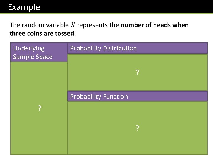
Example Underlying Sample Space { HHH, HHT, HTH, THH, ? THT, TTH, TTT } Probability Distribution 0 1 ? Probability Function ? 2 3

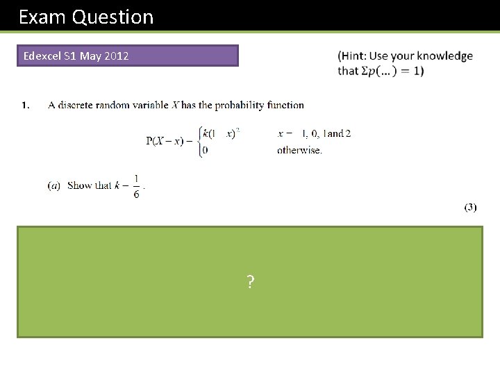
Exam Question Edexcel S 1 May 2012 ?

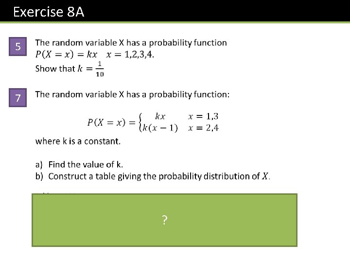
Exercise 8 A 5 7 ? x 1 2 P(X = x) 0. 125 3 4 0. 375

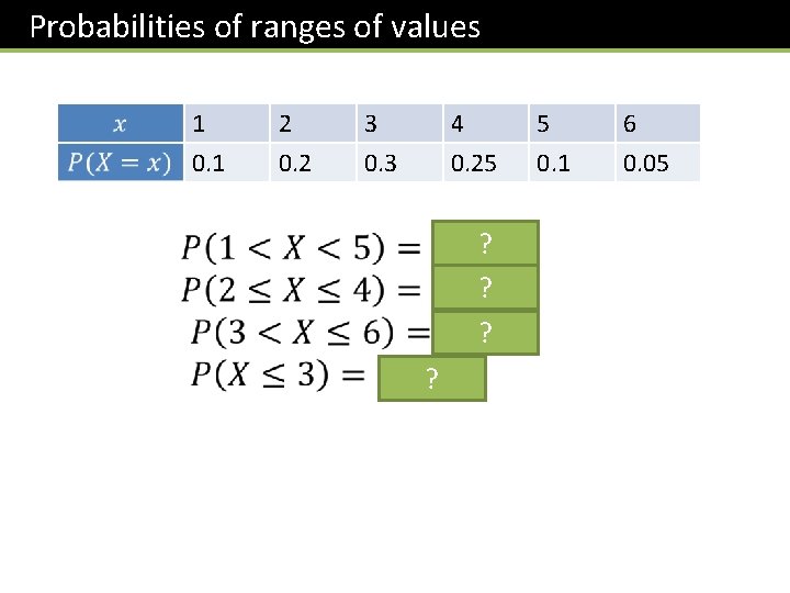
Probabilities of ranges of values 1 0. 1 2 0. 2 3 0. 3 4 0. 25 ? ? 5 0. 1 6 0. 05

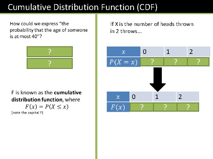
Cumulative Distribution Function (CDF) If X is the number of heads thrown in 2 throws. . . ? ? 0 0. 25 ? 1 0. 5? 1 0. 75 ? 2 0. 25 ? 2 1 ?

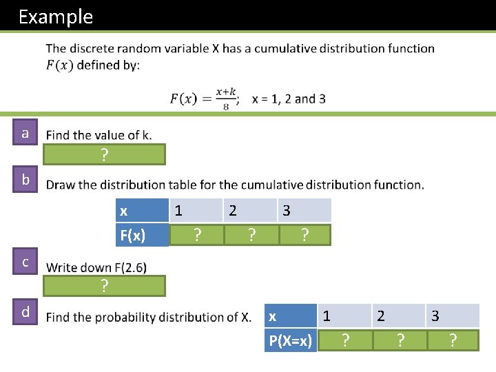
Example a ? b x F(x) 1 3/4? 2 7/8? 3 1 ? c ? d x 1 P(X=x) 3/4? 2 1/8? 3 1/8?

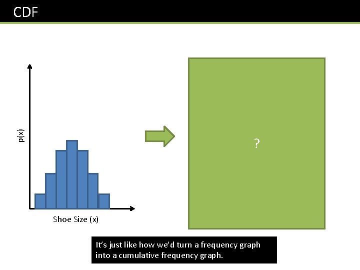
CDF F(x) p(x) 1 Shoe Size (x) ? Shoe Size (x) It’s just like how we’d turn a frequency graph into a cumulative frequency graph.

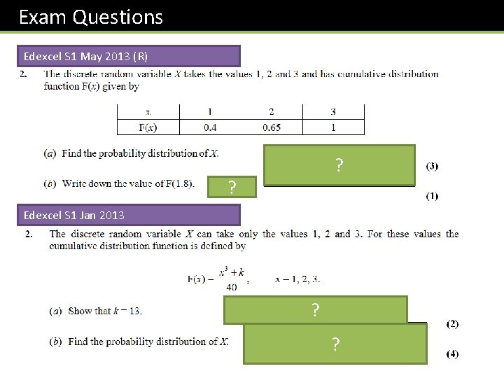
Exam Questions Edexcel S 1 May 2013 (R) = 0. 4 ? x 1 2 P(X = x) 0. 4 ? 0. 25 3 0. 35 Edexcel S 1 Jan 2013 F(3) = 1, so (27 + k)/40 = 1, . . . ? x 1 P(X = x) 0. 35 ? 2 3 0. 175 0. 475

Exercise 8 B Q 5 -8

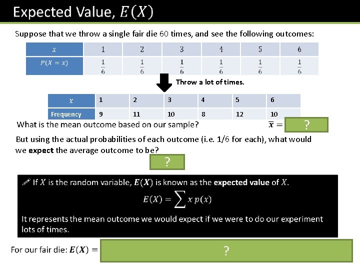
Suppose that we throw a single fair die 60 times, and see the following outcomes: Throw a lot of times. Frequency 1 2 3 4 5 6 9 11 10 8 12 10 ? But using the actual probabilities of each outcome (i. e. 1/6 for each), what would we expect the average outcome to be? 3. 5 ?

Quickfire E[X] Find the expected value of the following distributions (in your head!). 1 2 3 4 6 8 0. 1 0. 6 0. 3 0. 5 0. 25 ? ? Bro Tip: Suppose you treated the probabilities as frequencies then found the mean of the ‘frequency table’. What do you notice? 10 20 30 ? Bro Tip: If the distribution is ‘symmetrical’, i. e. both the outcomes and probabilities are symmetrical about the centre, then the expected value is this central value.

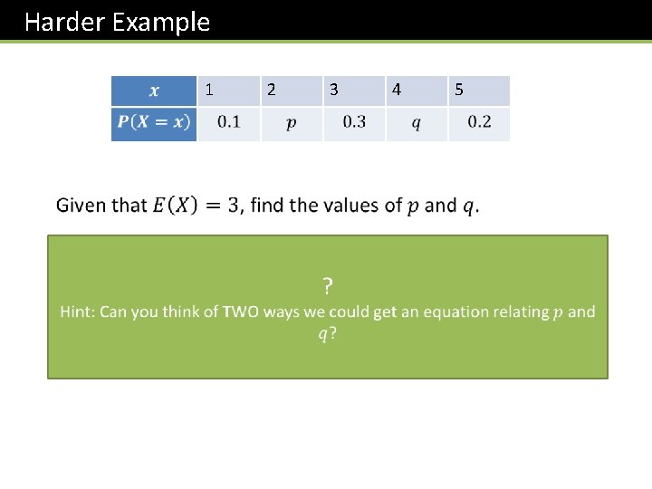
Harder Example 1 2 3 4 5

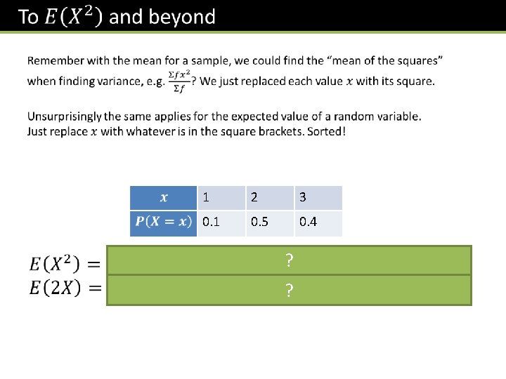
1 2 3 0. 1 0. 5 0. 4 ? ?

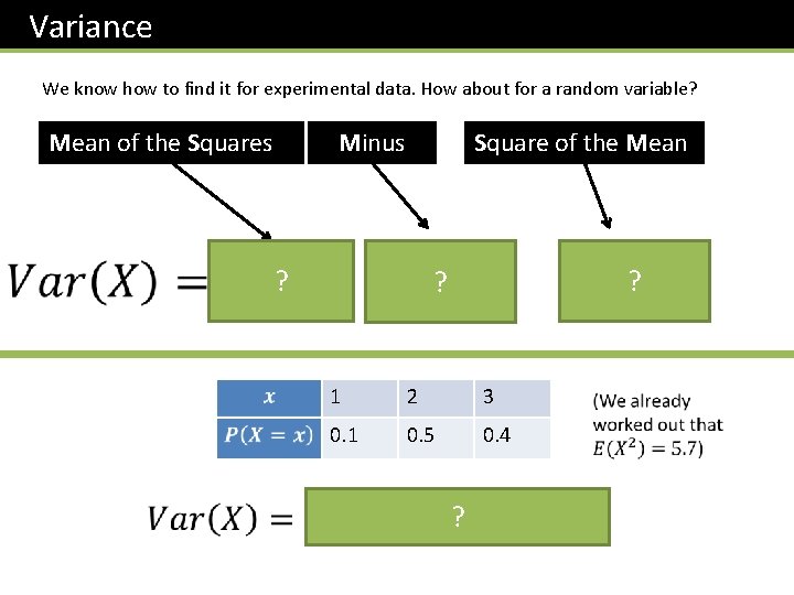
Variance We know how to find it for experimental data. How about for a random variable? Mean of the Squares Minus Square of the Mean – ? ? 1 2 3 0. 1 0. 5 0. 4 ? ?

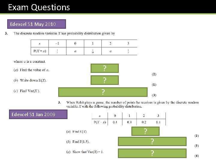
Exam Questions Edexcel S 1 May 2010 a = 1/4 ? = 1 ? 2 = 2. 1 E[X 2] = 3. 1 So Var[X] = 3. 1 – 1 ? Edexcel S 1 Jan 2009 ? = 1 = P(X <= 1. 5) = P(X <= 1) = 0. 7 ? 2 = 1 E[X 2] = 2. So Var[X] = 2 – 1 ?

Exercise 8 D

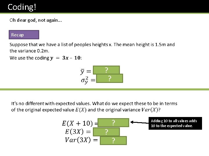
Coding! Oh dear god, not again. . . Recap ? ? ? Adding 10 to all values adds 10 to the expected value.

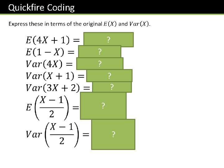
Quickfire Coding ? ? ? ?

Exercise 8 E 2 E[X] = 2, Var[X] = 6 Find a) E[3 X] = 3 E[X]? = 6 d) E[4 – 2 X] = 4 – 2 E[X] ? =0 f) Var[3 X + 1] = 9 Var[X] ? = 54 5 The random variable Y has mean 2 and variance 9. Find: a) E[3 Y+1] = 3 E[Y] ? +1=7 c) Var[3 Y+1] = 9 Var[Y] ? = 81 e) E[Y 2] = Var[Y] + ? E[Y]2 = 13 f) E[(Y-1)(Y+1)] = E[Y 2 – 1] = E[Y ? 2] – 1 = 12 Bro Exam Tip: This has come up in exams multiple times.

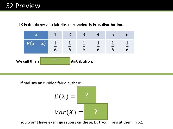
S 2 Preview If X is the throw of a fair die, this obviously is its distribution. . . We call this a discrete? uniform distribution. ? ? You won’t have exam questions on these, but you’ll revisit them in S 2.

Example ? ?