Running ABINIT Choi Hye Jin What is ABINIT

Running ABINIT Choi Hye Jin

What is ABINIT • total energy, charge density, electronic structure, forces of periodic solids and molecules (supercell geometry) • Density Functional Theory (DFT), Time-dependent DFT, Many-body perturbation theory (GW) • pseudopotentials, planewave basis, projector Augmented Waves • Geometry optimazation, dynamics • Linear responses, non-linear reponses (phonons, homogeneous electric field, stresses) • written mostly in F 90 • different utilities, automatic tests, documentation, tutorial… • +web site, mailing lists www. abinit. org ABINIT project PDF

ABINIT 특성 • “Free” or “Open Source” package • Distributed development : the groups (Europe, USA, Asia) • Reliable : More than 400 automated tests • Portable : Easy and frequent installation on more than 10 platforms • High-level coding and documentation : Explicit coding style, self-documentation • Many capabilities : Ground state, response functions, excited states • Easy to learn and use : Tutorial, examples, input metalanguage www. abinit. org ABINIT project PDF

Many capabilities www. abinit. org ABINIT project PDF
 log ABINIT")
External files in a ABINIT run Filenames Main input Pseudopotentials (previous results) log ABINIT Main output (other results) Results : density (_DEN), potential (_POT), wavefunctions (_WFK), density of states (_DOS)
 Optimization calculation Viewer UTIL - cut 3")
Contents SCF calculation Multi-test calculation (band structure) Optimization calculation Viewer UTIL - cut 3 d Input variables 6

Input files : ab. in, ab. files • Ab. in acell 10 10 10 rprim 1. 0 0. 0 1. 0 • Ab. files … … Ab. in ; main input file Ab. out ; main output file abi ; namely abi_WFK, see later abo ; will be written to abo_WFK tmp ; tmp_STATUS. . /Ps. P/14 si. psp ; pseudopotential files Pseudopotential file은 www. abinit. org 홈페이지에서 다양하게 제공하고 있으므로 다운받아서 이용할 수 있다.

Basic input variables #Definition of the unit cell acell 14. 0 2. 5037 angstrom # if 10 10 10 = 3*10 # unit default : Bohr # 1 bohr=0. 529177249 Angstroms rprim 1. 0 0. 0 1. 0 SCF calculation # dimensionless primitive transtations of peridic cell # each COLUMN of this array is one primitive translation. # fcc 0. 0 0. 5 bcc : -0. 5 0. 0 0. 5 -0. 5 Lesson 1 t 11. in , t 12. in

#Definition of the atom types ntypat 2 # n type of atom # There is two type of atom ( Boron, Nitrogen ) znucl 7 5 # The keyword "znucl" refers to the atomic # number of the possible type(s) of atom. # The pseudopotential(s) mentioned in the "files" file # must correspond to the type(s) of atom. #Definition of the atoms natom 20 # number of atoms # There are 20 atoms. typat 10*1 10*2 # type of atoms # 10 of N, 10 of B ( position order ) SCF calculation (ex) H 20 Ntypat 2 Znucl 1 8 Natom 3 Typat 1 1 2 = 2*1, 2
10. 02423 2) 3. 71173 3) 7. 61332 # This keyword indicate that")
xangst 1)10. 02423 2) 3. 71173 3) 7. 61332 # This keyword indicate that the location of the atoms # xcart ( cartesian coordinate – bohr ) # xred ( reduced coordinate ) # xangst ( cartesian coordinate – angstrom ) 6. 53087 1. 87750 4. 48514 1. 87801 N 9. 85125 1. 87753 10개의 cartesian angstrom coordinate … Znucl 7 5 11) 4. 82653 12)3. 18318 13)6. 17069 3. 56627 7. 23904 9. 93979 1. 87801 1. 87803 1. 87766 … SCF calculation typat 10*1 10*2 B 10개의 cartesian angstrom coordinate

#Definition of the planewave basis set ecut 45 Ry # Maximal kinetic energy cut-off, in Hartree # 'Ry ' => Rydberg (for energies) # 'e. V ' => electron-volts (for energies) # 'K ' => Kelvin (for energies) #Definition of the k-point grid kptopt 1 # KPoin. Ts OPTion # Option for the automatic generation of k points , taking into account the symmetry ngkpt 1 1 5 SCF calculation # Number of Grid points for K Poin. Ts generation # This is a 1 x 1 x 5 grid based on the primitive vectors

#Definition of the SCF procedure nstep 70 # Maximal number of SCF cycles # iterations toldfe 1. 0 d-6 # TOLerance on the Di. Fference of total Energy # Will stop when, twice in a row, the difference # between two consecutive evaluations of total # energy differ by less than toldfe (in Hartree) # toldfe, toldff, tolrff, tolvrs and tolwfr are aimed at the same goal diemac 2. 0 # Although this is not mandatory, it is worth to # precondition the SCF cycle. The model # dielectric function used as the standard # preconditioner is described in the "dielng“ # input variable section. SCF calculation
")
Spin-polarized calculation (H Nsppol 2 ; SPin-POLarized calculation ixc=0, 1, 7, 11 일때. atom) occopt 2 ; OCCupation OPtion nband 1 1 occ 1. 0 0. 0 ; spin up, down 에 대해서 따로 계산한다. ; occupation number for spin up & down state ; 1. 0 = half-occupied or other choices in special circumstances. spinat 0. 0 1. 0 ; SPIN for Atoms ; initial estimation of the spin on the atom # SCF input ……
 energy (hartree) = -0. 26414 Average Vxc")
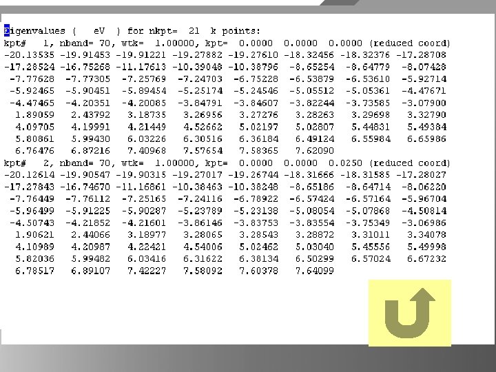
Output= t 15 o_EIG Fermi (or HOMO) energy (hartree) = -0. 26414 Average Vxc (hartree)= -0. 06898 Eigenvalues (hartree) for nkpt= 1 k points, SPIN UP: kpt# 1, nband= 1, wtk= 1. 00000, kpt= 0. 0000 (reduced coord) -0. 26414 Eigenvalues (hartree) for nkpt= 1 k points, SPIN DOWN: kpt# 1, nband= 1, wtk= 1. 00000, kpt= 0. 0000 (reduced coord) -0. 11109

t 12. in = rigid distance t 21. in =t 13. in+t 15. in t 23. in = rigid cell Multi-test input variable ndtest 21 ; 21개의 dataset xcart -0. 5 0. 0 xcart+ -0. 025 0. 0 getwfk -1 start point increment- start point 에서 xcart+ 값 만큼 변하면서 SCF 계산 ; 앞의 계산한 wavefuction 파일을 input 으로 읽겠다. 새로운 output wavefuction 파일을 만들 것이다. ; (ex) t 11 o_WFK ->t 12 i_W # SCF input variables…. .

21개의 data의 output data etotal 1 -1. 0368223891 E+00 etotal 2 -1. 0538645433 E+00 etotal 3 -1. 0674504851 E+00 etotal 4 -1. 0781904896 E+00 etotal 5 -1. 0865814785 E+00 etotal 6 -1. 0930286804 E+00 etotal 7 -1. 0978628207 E+00 etotal 8 -1. 1013539124 E+00 etotal 9 -1. 1037224213 E+00 etotal 10 -1. 1051483730 E+00 etotal 11 -1. 1057788247 E+00 etotal 12 -1. 1057340254 E+00 etotal 13 -1. 1051125108 E+00 etotal 14 -1. 1039953253 E+00 etotal 15 -1. 1024495225 E+00 etotal 16 -1. 1005310615 E+00 etotal 17 -1. 0982871941 E+00 fcart 1 -3. 8014412429 E-01 0. 00 fcart 2 -3. 0403170292 E-01 0. 00 fcart 3 -2. 4142950882 E-01 0. 00 fcart 4 -1. 8981857799 E-01 0. 00 fcart 5 -1. 4716521386 E-01 0. 00 fcart 6 -1. 1181997503 E-01 0. 00 fcart 7 -8. 2441144940 E-02 0. 00 fcart 8 -5. 7933488256 E-02 0. 00

ndtest 12 udtest 6 2 ; ndtest = 6 * 2 ecut 10 ; initial ecut = 10 Ha ecut+ 5 ; 10 Ha에서 5 Ha씩 늘려가면서 계산 ; 10, 15, … , 40 이렇게 2번. acell 8 8 8 ; initial cell = 8 8 8 Bohr acell+ 2 2 2 ; 2 2 2 bohr씩 늘려가면서 계산 # convergence with respect to the number of K points. ndtest 4 ngkpt 1 2 2 2 ngkpt 2 4 4 4 ngkpt 3 6 6 6 ngkpt 4 8 8 8 ; Number of Grid points for K Poin. Ts generation

Band structure calculation ndtest 2 ; first test is SCF calculation, second test is band calculation iscf -2 getden 2 -1 ; iscf = -2 일때만 가능하다. kptopt 2 -3 enunit 1 ; eigenenergies ‘e. V’ nband 2 8 ; 8개의 band ndivk 10 12 17 kptbounds 2 0. 5 0. 0 0. 5 1. 0 10 12 17 BNtube - ndtest
![Band structure output [pang_1 x@node 9 BNtube_ndtest 2]$ ls band. data BNtube. files BNtubeo_DS](http://slidetodoc.com/presentation_image_h2/d5b1f8bf28cf14dc6f4bcbc539c61037/image-19.jpg "Band structure output [pang_1 x@node 9 BNtube_ndtest 2]$ ls band. data BNtube. files BNtubeo_DS")
Band structure output [pang_1 x@node 9 BNtube_ndtest 2]$ ls band. data BNtube. files BNtubeo_DS 1_DEN BNtubeo_DS 1_WFK BNtubeo_DS 2_EIG 2 band. f 90 band. ps BNtube. ndtest. in BNtube. ndtest. out BNtubeo_DS 1_EIG BNtubeo_DS 2_DEN BNtubeo_DS 2_WFK Gband. in [pang_1 x@node 9 BNtube_ndtest 2]$ vi BNtubeo_DS 2_EIG Eigenvalue file Band. ps band. data EIG 2 band. f 90 Gband. in

BNtubeband data ps file viewer program Ghost viewer

Optimization input variable #optimize interatomic distance ionmov 3 ; Broyden algorithm ntime 10 ; Broyden “time steps” tolmxf 5. 0 d-4 ; stopping cristerion geometry opt. ; residual force < tolmxf toldff 5. 0 d-5 ; the difference two consecutive evaluation of forces ( Ha/bohr ) #SCF input variables ….

#optimization of lattice parameter optcell 1 ; optimisation of volume only (do not modify rprim, and allow an homogeneous dilatation of the three components of acell) ionmov 3 ; Broyden algorithm ecutsm 0. 5 ; performing relaxation of unit cell size and shape (non-zero optcell). Using a non-zero ecutsm, the total energy curves as a function of ecut, or acell, can be smoothed, keeping consistency with the stress. The recommended value is 0. 5 Ha.
 acell 6")
N 2 excited state ( LDA / #Common ndtset 2 TDLDA ) acell 6 2*5 Angstrom #DATASET 1 SCF iscf 1 5 tolwfr 1 1. 0 d-15 nband 1 5 prtden 1 1 getwfk 1 0 #DATASET 2 TDDFT iscf 2 -1 tolwfr 2 1. 0 d-9 nband 2 12 getden 2 1 getwfk 2 1 boxcenter 3*0. 0 d 0 diemac 1. 0 d 0 diemix 0. 5 d 0 ecut 25 ixc 7 Time-Dependent Density Functional Theory (Casida's approach)

Output data files – N 2 excited state ttddft_1. in ttddft_x. files ttddft_1. out ttdft_1 o_DS 1_EIG ttdft_1_TDEXCIT ttdft_1 o_DS 1_DDB ttdft_1 o_DS 1_WFK ttdft_1 o_DS 1_DEN ttdft_1 o_DS 2_EIG

Viewer UTIL – cut 3 d Abinit 을 이용하여 density, wavefuction 등을 계산하였다. 계산한 분자나 고체에 대하여 charge density나 wavefunction, STM image 등 을 그려보고자 할 때 “cut 3 d” 를 이용하면 open. DX, xcrysden 등을 이용하여 그려볼 수 있다. [pang_1 x@node 9 opt]$ ls benzene_bzo_EIG benzene_bzo_TIM 2_DEN benzene. opt. in benzene_bzo_TIM 0_DEN benzene_bzo_WFK benzene_bzo_DDB benzene_bzo_TIM 1_DEN benzene. files benzene. opt. out
![[pang@node 1 benzene]$ ls benzene_bzo_DEN [pang@node 1 benzene]$ cut 3 d. Version 5. 3.](http://slidetodoc.com/presentation_image_h2/d5b1f8bf28cf14dc6f4bcbc539c61037/image-27.jpg "[pang@node 1 benzene]$ ls benzene_bzo_DEN [pang@node 1 benzene]$ cut 3 d. Version 5. 3.")
[pang@node 1 benzene]$ ls benzene_bzo_DEN [pang@node 1 benzene]$ cut 3 d. Version 5. 3. 4 of CUT 3 D. (sequential version, prepared for a x 86_64_linux_intel computer) What is the name of the 3 D function (density, potential or wavef) file ? benzene_bzo_DEN => Your 3 D function file is : benzene_bzo_DEN Does this file contain formatted 3 D ASCII data (=0) or unformatted binary header + 3 D data (=1) ? 1 ============================ ECHO of the ABINIT file header First record : . codvsn, headform, fform = 5. 3. 5 53 52 Cut 3 d - Density - xcrysden

What is your choice ? Type: 0 => exit 5 => 3 D formatted data (output the bare 3 D data - one column) 6 => 3 D indexed data (bare 3 D data, preceeded by 3 D index) 7 => 3 D Molekel formatted data 8 => 3 D data with coordinates (tecplot ASCII format) 9 => output. xsf file for XCrys. Den 10 => output. dx file for Open. Dx 11 => compute atomic charge using the Hirshfeld method 12 => Net. CDF file 9 Your choice is 9 Enter the name of an output file: benzene The name of your file is : benzene Cut 3 d - Density - xcrysden

Do you want to shift the grid along the x, y or z axis (y/n)? n Task 9 has been done ! 0 More analysis of the 3 D file ? (1=default=yes, 0=no) Thank you for using me [pang@node 1 benzene]$ ls benzene_bzo_DEN Xcrysden file Cut 3 d - Density - xcrysden
![[pang@node 1 benzene]$ ls benzene_bzo_WFK [pang@node 1 benzene]$ cut 3 d. Version 5. 3.](http://slidetodoc.com/presentation_image_h2/d5b1f8bf28cf14dc6f4bcbc539c61037/image-30.jpg "[pang@node 1 benzene]$ ls benzene_bzo_WFK [pang@node 1 benzene]$ cut 3 d. Version 5. 3.")
[pang@node 1 benzene]$ ls benzene_bzo_WFK [pang@node 1 benzene]$ cut 3 d. Version 5. 3. 4 of CUT 3 D. (sequential version, prepared for a x 86_64_linux_intel computer). Copyright (C) 1998 -2007 ABINIT group. CUT 3 D comes with ABSOLUTELY NO WARRANTY. It is free software, and you are welcome to redistribute it under certain conditions (GNU General Public License, see ~abinit/COPYING or http: //www. gnu. org/copyleft/gpl. txt). What is the name of the 3 D function (density, potential or wavef) file ? benzene_bzo_WFK => Your 3 D function file is : benzene_bzo_WFK Cut 3 d-Wavefuction - xcrysden
 or unformatted binary header")
Does this file contain formatted 3 D ASCII data (=0) or unformatted binary header + 3 D data (=1) ? 1 1 => Your file contains unformatted binary header + 3 D data The information it contains should be sufficient. cut 3 d : read file benzene_bzo_WFK from unit number 19. ============ ECHO of the ABINIT file header First record : . codvsn, headform, fform = 5. 3. 5 53 2 8 9 10 11 12 1. 267490 E+01 8. 321816 E+00 1. 267490 E+01 8. 321819 E+00 1. 049835 E+01 8. 473461 E+00 7. 138094 E+00 8. 473461 E+00 7. 138095 E+00 7. 805777 E+00 This file is a WF file. Cut 3 d-Wavefuction - xcrysden 1. 282579 E+01 1. 545462 E+01 1. 676905 E+01

If you want to analyze one wavefunction, type 0 If you want to construct Wannier-type Localized Orbitals, type 2 0 You typed 0 => Your k-point is : 1 For which band ? (1 to 17) 11 => Your band number is : 11 => Your spin polarisation number is : 1 Do you want the atomic analysis for this state : (kpt, band)= ( 1 11)? If yes, enter the radius of the atomic spheres, in bohr If no, enter 0 0 You entered ratsph= 0. 0000 Bohr Cut 3 d-Wavefuction - xcrysden

What is your choice ? Type: 0 => exit to k-point / band / spin-pol loop 1 => 3 D formatted real and imaginary data (output the bare 3 D data - two column, R, I) 2 => 3 D formatted real data (output the bare 3 D data - one column) 9 => 3 D Data Explorer formatted data (Only the Imaginary file) 10 => 3 D Data Explorer formatted data and position files 11 => XCrysden formatted data and position files 12 => Net. CDF data and position file 13 => XCrysden/VENUS wavefunction real data 10 Your choice is 10 Enter the root of an output file: 11 The root of your file is : 11 The corresponding filename is : 11_k 1_b 11_s 1 Cut 3 d-Wavefuction - xcrysden

Give 5 files of formatted data The files are ready to be use with Data Explorer The eigenvalues and occupations numbers are in comments of the two data files The name of your data files is : 11_k 1_b 11_s 1 Real. dx for the real part, 11_k 1_b 11_s 1 Imag. dx for the imaginary part. Give the lattice file, 11_LATTICE_VEC. dx Give the atoms positions file, 11_ATOM_POS. dx Give the enveloppe of the cell file, 11_UCELL_FRAME. dx Task 0 10 has been done ! Run interpolation again? (1=default=yes, 0=no) Thank you for using me Cut 3 d-Wavefuction - xcrysden
![[pang@node 1 benzene]$ ls 11_ATOM_POS. dx 11_k 1_b 11_s 1 Imag. dx 11_k 1_b](http://slidetodoc.com/presentation_image_h2/d5b1f8bf28cf14dc6f4bcbc539c61037/image-35.jpg "[pang@node 1 benzene]$ ls 11_ATOM_POS. dx 11_k 1_b 11_s 1 Imag. dx 11_k 1_b")
[pang@node 1 benzene]$ ls 11_ATOM_POS. dx 11_k 1_b 11_s 1 Imag. dx 11_k 1_b 11_s 1 Real. dx 11_LATTICE_VEC. dx 11_UCELL_FRAME. dx benzene_bzo_WFK [pang@comphys benzene]$ ls 11_ATOM_POS. dx 11_k 1_b 11_s 1 Real. dx DX 2 Xcry. x 11_LATTICE_VEC. dx 12_ATOM_POS. dx 11_k 1_b 11_s 1 Imag. dx 11_UCELL_FRAME. dx [pang@comphys benzene]$. /DX 2 Xcry. x Enter the name of DX file from ABinit cut 3 d 11_k 1_b 11_s 1 Real. dx Enter the name of DX pos file from ABinit cut 3 d 11_ATOM_POS. dx hereihave datmax 1 19. 38791 N 1=== 100 N 2=== 80 N 3=== 135 origin 0. 0000000 E+00 a 3 0. 0000000 E+00 0. 1256693 a 2 0. 0000000 E+00 0. 1282660 0. 0000000 E+00 a 1 0. 1311099 0. 0000000 E+00 hereihave max 19. 38791 Cut 3 d-Wavefuction - xcrysden
![[pang@comphys benzene]$ ls 11_ATOM_POS. dx 11_k 1_b 11_s 1 Real. dx 11. xsf DX](http://slidetodoc.com/presentation_image_h2/d5b1f8bf28cf14dc6f4bcbc539c61037/image-36.jpg "[pang@comphys benzene]$ ls 11_ATOM_POS. dx 11_k 1_b 11_s 1 Real. dx 11. xsf DX")
[pang@comphys benzene]$ ls 11_ATOM_POS. dx 11_k 1_b 11_s 1 Real. dx 11. xsf DX 2 Xcry. x 11_LATTICE_VEC. dx 11_k 1_b 11_s 1 Imag. dx 11_UCELL_FRAME. dx [pang@comphys benzene]$ ls 11_ATOM_POS. dx 11. jpg 11_k 1_b 11_s 1 Imag. dx 11_k 1_b 11_s 1 Real. dx 11_LATTICE_VEC. dx 11_UCELL_FRAME. dx 11. xsf 12. xsf 13. xsf 14. xsf 15. xsf 16. xsf 17. xsf DX 2 Xcry. x [pang@comphys benzene]$ xcrysden Cut 3 d-Wavefuction - xcrysden
 energy (e. V) = -6. 22492 Average Vxc (e. V)=")
Benzene_opt_EIG Fermi (or HOMO) energy (e. V) = -6. 22492 Average Vxc (e. V)= -0. 75919 Eigenvalues ( e. V ) for nkpt= 1 k points: kpt# 1, nband= 17, wtk= 1. 00000, kpt= 0. 0000 (reduced coord) -20. 94578 -18. 08572 -18. 08553 -14. 49398 -14. 49396 -12. 67527 -10. 75678 -10. 75498 -9. 96569 -9. 96542 -8. 99858 -7. 94717 -7. 94680 -6. 22498 -6. 22492 -1. 07861 -1. 07810

Benzene – 11 ~ 15 state 11= -8. 99858 e. V 12= -7. 94717 e. V 14= -6. 22498 e. V 15= -6. 22492 e. V 13= -7. 94680 e. V

Tip !!! enunit ; default = Ha, 1=e. V prtdos ; Provide output of Density of States 1 : Can either use a smearing technique 2 : tetrahedron method 3 : Local Density of States inside a sphere centered on an atom, as well as the angular-momentum projected DOS, in the same sphere. The resolution of the linear grid of energies for which the DOS is computed can be tuned thanks to dosdeltae.
. A")
ixc ; Integer for e. Xchange-Correlation choice ; Default is ixc=1 (Teter parameterization). A warning is issued if this is not the case. However, the choices ixc=1, 2, 3 and 7 are fits to the same data, from Ceperley-Alder, and are rather similar, at least for spin-unpolarized systems. The choice between the LDA and the LSDA (or between the GGA and spin-GGA) is governed by the value of nsppol (see below). occopt ; set the OCCupation OPTion of electronic levels ; =1 (semiconductor), =3 … 7 (metals)

prtstm ; If set to 1 or a larger value, provide output of the electron density in real space rho(r), made only from the electrons close to the Fermi energy, in a range of energy (positive or negative), determined by the (positive or negative, but non-zero) value of the STM bias stmbias. This is a very approximate way to obtain STM profiles : one can choose an equidensity surface, and consider that the STM tip will follow this surface. tphysel ; Temperature (PHYSical) of the ELectrons ; Gives, in Hartree, the physical temperature of the system, in case occopt=4, 5, 6, or 7. Can be specified in Ha (the default), Ry, e. V or Kelvin, since ecut has the 'ENERGY' characteristics. 0. 001 Ha = 27. 2113845 me. V = 315. 773 Kelvin.
 and Langevin dynamics (ionmove=9) ,")
mdftemp ; Molecular Dynamics Final Temperature ; Nose-Hoover thermostat(ionmov=8) and Langevin dynamics (ionmove=9) , in Kelvin. mditemp ; Molecular Dynamics Initial Temperature mdwall ; Molecular Dynamics WALL location ; Default is 10000. 0 bohr location (atomic units) of walls on which the atoms will bounce back. When ionmov=6, 7. 8, 9) ntime ; Number of TIME steps ; Default is 5. MD timesteps or Broyden structural optimization steps. Ignored ionmov=0 Molecular Dynamics
 ; default = 3*natom 0’s.")
Vel ; VELoity , real array vel (3, atom) ; default = 3*natom 0’s. starting velocities of atoms, in cartesian coordinates. In bohr/atomic time unit) ionmov =8 (Nose thermostat), vel is not initialized, a random initial velocity giving the right kinetic energy will be generated. Molecular Dynamics

ionmov 0 => do not move ions = default; 1 => move atoms using molecular dynamics with optional viscous damping (friction linearly proportional to velocity). 2 , 3 => conduct structural optimization using the Broyden-Fletcher. Goldfarb-Shanno minimization (BFGS). 4 => conjugate gradient algorithm for simultaneous optimization of potential and ionic degrees of freedom. 5 => Simple relaxation of ionic positions according to (converged) forces. . 6 => Molecular dynamics using the Verlet algorithm 7 => Quenched Molecular dynamics using the Verlet algorithm, and stopping each atom for which the scalar product of velocity and force is negative. 8 => Molecular dynamics with Nose-Hoover thermostat, using the Verlet algorithm. initial temperature (mditemp), the final temperature (mdftemp), and thermostat mass (noseinert). 9 => Langevin molecular dynamics. the friction coefficient (friction). 12 => Isokinetic ensemble molecular dynamics.
 =1 => get the largest")
iscf ( v 5. 3 – 5, 14 ) =1 => get the largest eigenvalue of the SCF cycle =2 => SCF cycle, simple mixing of the potential =3 => SCF cycle, Anderson mixing of the potential =4 => SCF cycle, Anderson mixing of the potential based on the two previous iterations =5 => SCF cycle, CG based on the minim. of the energy with respect to the potential =7 => SCF cycle, Pulay mixing of the potential based on the npulayit previous iterations =12 => SCF cycle, simple mixing of the density =13 => SCF cycle, Anderson mixing of the density =14 => SCF cycle, Anderson mixing of the density based on the two previous iterations =15 => SCF cycle, CG based on the minim. of the energy with respect to the density =17 => SCF cycle, Pulay mixing of the density based on the npulayit previous iterations
 crystalline silicon (fcc) (ex) bcc rprim 0. 0 0. 5 rprim -0.")
rprim (ex) crystalline silicon (fcc) (ex) bcc rprim 0. 0 0. 5 rprim -0. 5 0. 0 0. 5 -0. 5 xred 0. 0 ¼ ¼ ¼ nshiftk 4 nshiftk 2 shiftk 0. 25 -0. 25 Shiftk 0. 5 0. 0 0. 5

Nsppol ; Number of SPin POLarization Give the number of INDEPENDENT spin polarisations. Can take the values 1 or 2. If nsppol=1(default), one has an unpolarized calculation (nspinor=1, nspden=1) or an antiferromagnetic system (nspinor=1, nspden=2), or a calculation in which spin up and spin down cannot be disantengled (nspinor=2), that is, either non-collinear magnetism or presence of spin-orbit coupling, for which one needs spinor wavefunctions. If nsppol=2, one has a spin-polarized (collinear) calculation with separate and different wavefunctions for up and down spin electrons for each band k point. Compatible only with nspinor=1, nspden=2.

diemac • A rough knowledge of the macroscopic dielectric constant diemac of the system is a useful help to speed-up the SCF procedure. • • • metals, simply put diemac to a very large value (the default 106 is OK) silicon, use 12. 0. A similar value is likely to work well for other semiconductors wider gap insulators, use 2. 0. . . 4. 0 molecules in an otherwise empty big box, try 1. 5. . . 3. 0 highly polarisable part and some vacuum are rather badly treated by the model dielectric function. One has to use the "extrapolar" technique, activated by the input variable iprcel.
 NOTE that a choice of nstep=0 is permitted;")
Nstep (Number of self-consistent field STEPS) NOTE that a choice of nstep=0 is permitted; this will either read wavefunctions from disk (with irdwfk=1 or irdwfq=1, or non-zero getwfk or getwfq in the case of multidataset) and compute the density, the total energy and stop, or else (with all of the above vanishing) will initialize randomly the wavefunctions and compute the resulting density and total energy. This is provided for testing purposes. Also NOTE that nstep=0 with irdwfk=1 will exactly give the same result as the previous run only if the later is done with iscf<10 (potential mixing). One can output the density by using prtden. The forces and stress tensor gets computed with nstep=0.

kptopt • • • 0=> read directly nkpt, kptnrm and wtk (corresponds to the usage before version 2. 1) One can use the kptgen utility to produce these input data. 1=> rely on ngkpt or kptrlatt, as well as on nshiftk and shiftk to set up the k points. Take fully into account the symmetry to generate the k points in the Irreducible Brillouin Zone only. (This is the usual mode for GS calculations) 2=> rely on ngkpt or kptrlatt, as well as on nshiftk and shiftk to set up the k points. Take into account only the time-reversal symmetry : k points will be generated in half the Brillouin zone. (This is to be used when preparing or executing a RF calculation at q=(0 0 0) ) 3=> rely on ngkpt or kptrlatt, as well as on nshiftk and shiftk to set up the k points. Do not take into account any symmetry : k points will be generated in the full Brillouin zone. (This is to be used when preparing or executing a RF calculation at non -zero q ) (4=> has been replaced by negative values in version 2. 3 ) A negative value => rely on kptbounds, and ndivk to set up a band structure calculation along different lines (allowed only for iscf==-2). The absolute value of kptopt gives the number of segments of the band structure.
- Slides: 50