ROYAL METEOROLOGICAL INSTITUTE OF BELGIUM ROYAL OBSERVATORY OF

ROYAL METEOROLOGICAL INSTITUTE OF BELGIUM ROYAL OBSERVATORY OF BELGIUM ROYAL BELGIAN INSTITUTE FOR SPACE AERONOMY MAX PLANCK INSTITUTE FOR CHEMISTRY SOLAR-TERRESTRIAL CENTRE OF EXCELLENCE 1 2 3 4 5 A world-wide analysis of the time variability of Integrated Water Vapour, based on groundbased GNSS and GOMESCIA satellite retrievals, and with reanalyses as auxiliary tools R. Van Malderen 1, 5, E. Pottiaux 2, 5, J. Legrand 2, H. Brenot 3, 5, S. Beirle 4, T. Wagner 4, H. De Backer 1, and C. Bruyninx 2, 5 GNSS 4 SWEC workshop, ESTEC, 21 -23/02/2017

ROB Outline 1. Recapitulation & introduction 2. Model setup 3. Seasonal behaviour 4. Model performance 5. Conclusions & Perspectives GNSS 4 SWEC workshop ESTEC, Noordwijk (NL) 21 -23 February 2017

Recapitulation & introduction Model setup Seasonal behaviour Model Performance ROB Datasets IGS repro 1 ◦ homogenous data processing from January 1995 to April 2011 ◦ data taken at 0 h & 12 h ( future: also at 6 h & 18 h) ◦ ZTD IWV by means of ERA-interim/NCEPNCAR (Ps from surface, Tm from vertical levels) ◦ screening: STD < 5 mm (NOT O. Bock’s screening and outlier removal applied to reference IGS repro 1 dataset in homogenization activity) ◦ not homogenized ERA-interim/NCEPNCAR reanalyses ◦ IWV from surface fields, corrected to IGS station height ◦ at 0 h & 12 h GOMESCIA ◦ GOME/SCIAMACHY/GOME-2 satellite overpass measurements at IGS stations ◦ (1996 - ongoing) ◦ not homogenized product ( new climate product will be evaluated) GNSS 4 SWEC workshop ESTEC, Noordwijk (NL) 21 -23 February 2017

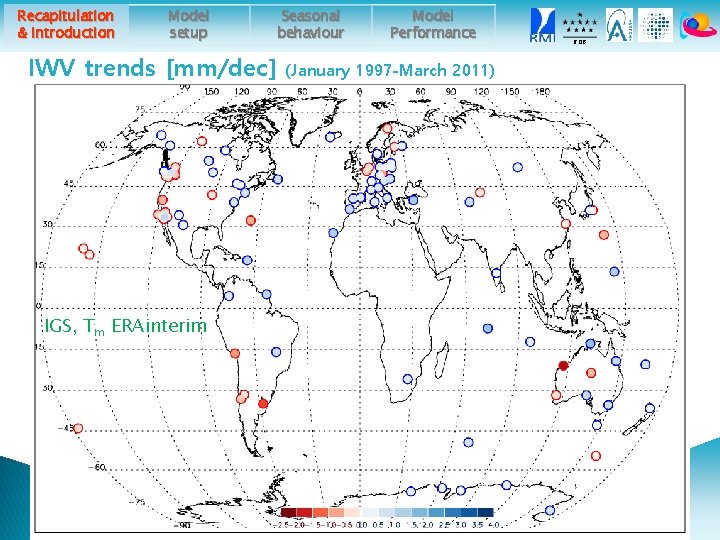
Recapitulation & introduction Model setup IWV trends [mm/dec] IGS, Tm ERAinterim Seasonal behaviour Model Performance (January 1997 -March 2011) ROB

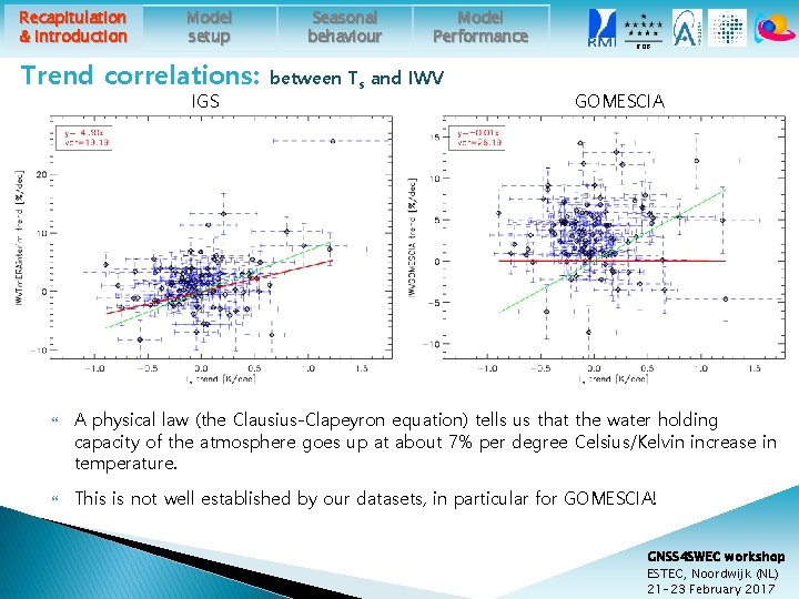
Recapitulation & introduction Model setup Trend correlations: IGS Seasonal behaviour Model Performance between Ts and IWV ROB GOMESCIA A physical law (the Clausius-Clapeyron equation) tells us that the water holding capacity of the atmosphere goes up at about 7% per degree Celsius/Kelvin increase in temperature. This is not well established by our datasets, in particular for GOMESCIA! GNSS 4 SWEC workshop ESTEC, Noordwijk (NL) 21 -23 February 2017

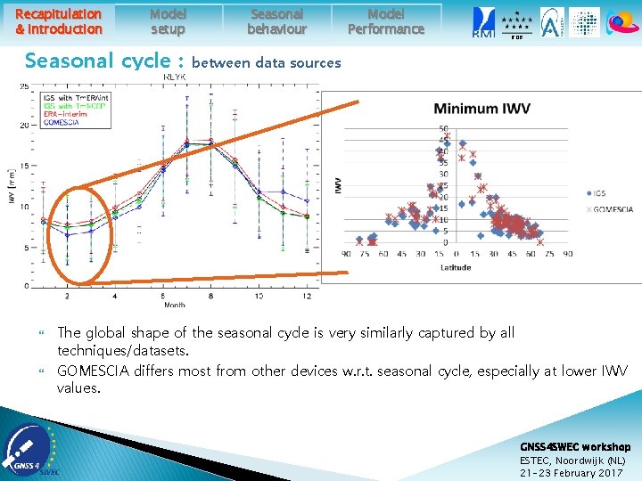
Recapitulation & introduction Model setup Seasonal cycle : Seasonal behaviour Model Performance ROB between data sources The global shape of the seasonal cycle is very similarly captured by all techniques/datasets. GOMESCIA differs most from other devices w. r. t. seasonal cycle, especially at lower IWV values. GNSS 4 SWEC workshop ESTEC, Noordwijk (NL) 21 -23 February 2017

Recapitulation & introduction Model setup Seasonal behaviour Model Performance ROB Main focus in this presentation: What are the main drivers of the seasonal variability and long-term time behaviour of the IWV time series? How can this scientific question be assessed? ◦ running climate models and study the underlying processes (e. g. validation of climate models with GNSS IWV retrievals see e. g. talk by Julie Berckmans) ◦ building empirical “models”, based on representations (=time series, in particular monthly means) of circulation patterns (e. g. ENSO) and lower-atmospheric oscillations (e. g. NAO) GNSS 4 SWEC workshop ESTEC, Noordwijk (NL) 21 -23 February 2017

Recapitulation & introduction Model setup Seasonal behaviour Model Performance ROB Main focus in this presentation: What are the main drivers of the seasonal variability and long-term time behaviour of the IWV time series? How can this scientific question be assessed? ◦ running climate models and study the underlying processes (e. g. validation of climate models with GNSS IWV retrievals see e. g. talk by Julie Berckmans) ◦ building empirical “models”, based on representations (=time series, in particular monthly means) of circulation patterns (e. g. ENSO) and lower-atmospheric oscillations (e. g. NAO) stepwise multiple linear regression GNSS 4 SWEC workshop ESTEC, Noordwijk (NL) 21 -23 February 2017

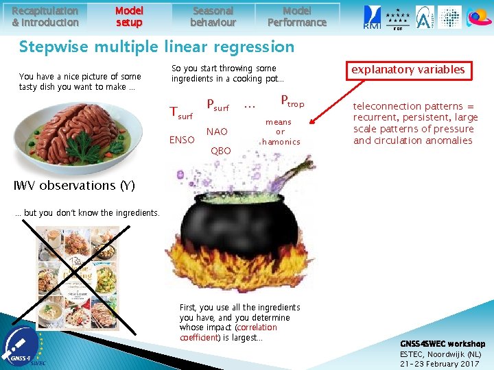
Recapitulation & introduction Model setup Model Performance Seasonal behaviour ROB Stepwise multiple linear regression You have a nice picture of some tasty dish you want to make … So you start throwing some ingredients in a cooking pot… Tsurf ENSO Psurf NAO QBO . . . Ptrop means or hamonics explanatory variables teleconnection patterns = recurrent, persistent, large scale patterns of pressure and circulation anomalies IWV observations (Y) … but you don’t know the ingredients. First, you use all the ingredients you have, and you determine whose impact (correlation coefficient) is largest… GNSS 4 SWEC workshop ESTEC, Noordwijk (NL) 21 -23 February 2017

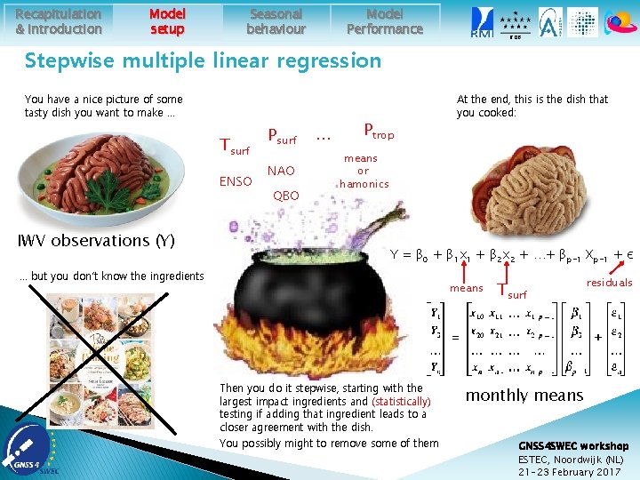
Recapitulation & introduction Model setup Model Performance Seasonal behaviour ROB Stepwise multiple linear regression You have a nice picture of some tasty dish you want to make … Tsurf ENSO IWV observations (Y) Psurf NAO QBO . . . Ptrop At the end, this is the dish that you cooked: means or hamonics Y = β 0 + β 1 x 1 + β 2 x 2 + …+ βp-1 Xp-1 + ε … but you don’t know the ingredients means Then you do it stepwise, starting with the largest impact ingredients and (statistically) testing if adding that ingredient leads to a closer agreement with the dish. You possibly might to remove some of them Tsurf residuals monthly means GNSS 4 SWEC workshop ESTEC, Noordwijk (NL) 21 -23 February 2017

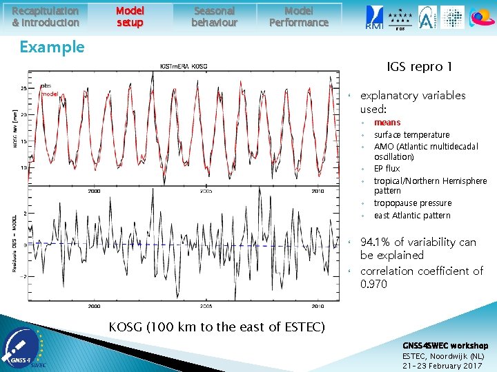
Recapitulation & introduction Model setup Seasonal behaviour Model Performance ROB Example IGS repro 1 explanatory variables used: ◦ ◦ ◦ ◦ means surface temperature AMO (Atlantic multidecadal oscillation) EP flux tropical/Northern Hemisphere pattern tropopause pressure east Atlantic pattern 94. 1% of variability can be explained correlation coefficient of 0. 970 KOSG (100 km to the east of ESTEC) GNSS 4 SWEC workshop ESTEC, Noordwijk (NL) 21 -23 February 2017

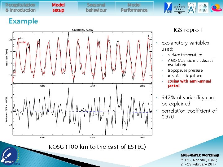
Recapitulation & introduction Model setup Seasonal behaviour Model Performance ROB Example IGS repro 1 explanatory variables used: ◦ ◦ ◦ surface temperature AMO (Atlantic multidecadal oscillation) tropopause pressure east Atlantic pattern cosine with semi-annual period 94. 2% of variability can be explained correlation coefficient of 0. 970 KOSG (100 km to the east of ESTEC) GNSS 4 SWEC workshop ESTEC, Noordwijk (NL) 21 -23 February 2017

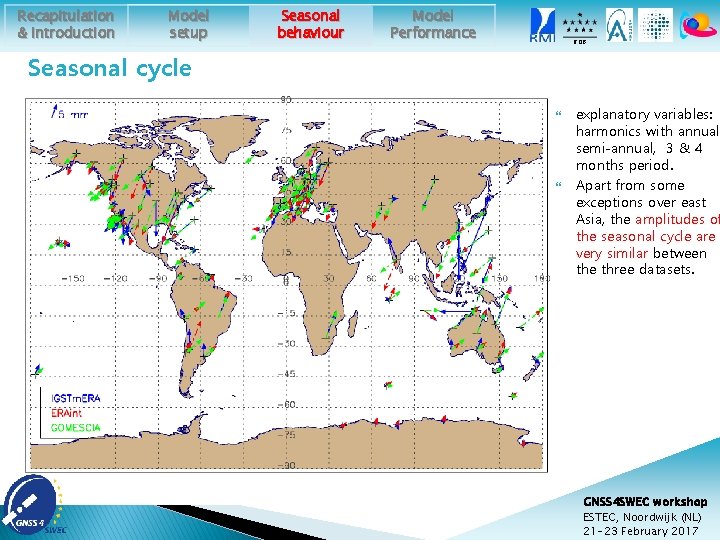
Recapitulation & introduction Model setup Seasonal behaviour Model Performance ROB Seasonal cycle explanatory variables: harmonics with annual, semi-annual, 3 & 4 months period. Apart from some exceptions over east Asia, the amplitudes of the seasonal cycle are very similar between the three datasets. GNSS 4 SWEC workshop ESTEC, Noordwijk (NL) 21 -23 February 2017

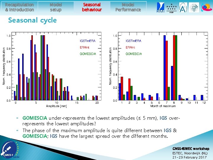
Recapitulation & introduction Model setup Seasonal behaviour Model Performance ROB Seasonal cycle GOMESCIA under-represents the lowest amplitudes (≤ 5 mm), IGS overrepresents the lowest amplitudes? The phase of the maximum amplitude is quite different between IGS & GOMESCIA; IGS have the largest spread over the different months. GNSS 4 SWEC workshop ESTEC, Noordwijk (NL) 21 -23 February 2017

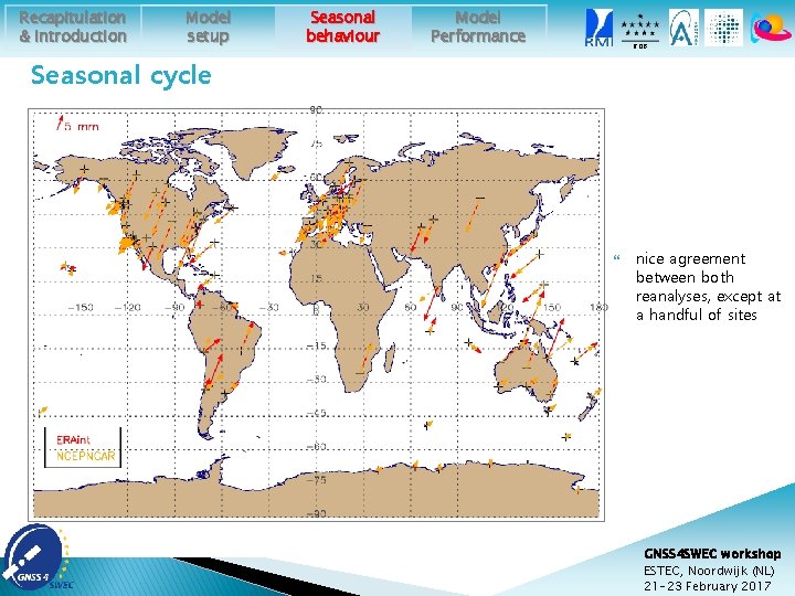
Recapitulation & introduction Model setup Seasonal behaviour Model Performance ROB Seasonal cycle nice agreement between both reanalyses, except at a handful of sites GNSS 4 SWEC workshop ESTEC, Noordwijk (NL) 21 -23 February 2017

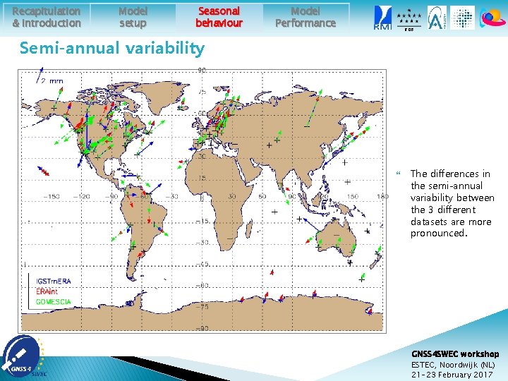
Recapitulation & introduction Model setup Seasonal behaviour Model Performance ROB Semi-annual variability The differences in the semi-annual variability between the 3 different datasets are more pronounced. GNSS 4 SWEC workshop ESTEC, Noordwijk (NL) 21 -23 February 2017

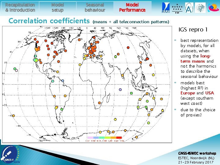
Recapitulation & introduction Model setup Seasonal behaviour Correlation coefficients Model Performance ROB (means + all teleconnection patterns) IGS repro 1 best representation by models, for all datasets, when using the longterm means and not the harmonics to describe the seasonal behaviour models best (highest R²) in Europe and USA (except southern west coast) due to the choice of proxies? GNSS 4 SWEC workshop ESTEC, Noordwijk (NL) 21 -23 February 2017

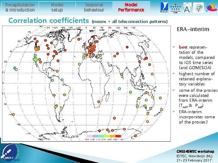
Recapitulation & introduction Model setup Seasonal behaviour Correlation coefficients Model Performance ROB (means + all teleconnection patterns) ERA-interim best representation of the models, compared to IGS time series (and GOMESCIA) highest number of retained explanatory variables some of the proxies were calculated from ERA-interim (Tsurf & Psurf) ERA-interim incorporates some of the proxies? GNSS 4 SWEC workshop ESTEC, Noordwijk (NL) 21 -23 February 2017

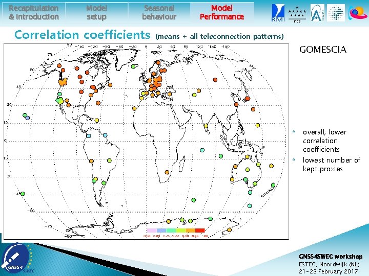
Recapitulation & introduction Model setup Seasonal behaviour Correlation coefficients Model Performance ROB (means + all teleconnection patterns) GOMESCIA overall, lower correlation coefficients lowest number of kept proxies GNSS 4 SWEC workshop ESTEC, Noordwijk (NL) 21 -23 February 2017

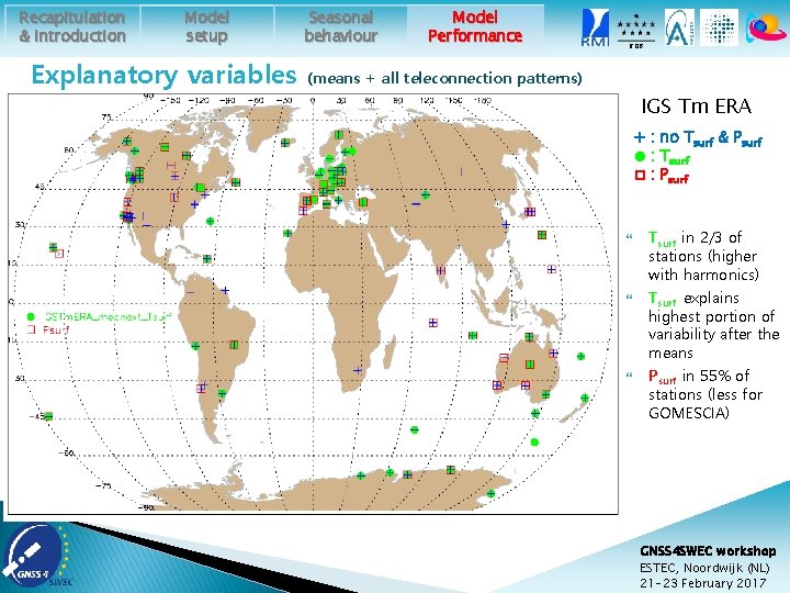
Recapitulation & introduction Model setup Explanatory variables Seasonal behaviour Model Performance ROB (means + all teleconnection patterns) IGS Tm ERA + : no Tsurf & Psurf ● : Tsurf □ : Psurf Tsurf in 2/3 of stations (higher with harmonics) Tsurf explains highest portion of variability after the means Psurf in 55% of stations (less for GOMESCIA) GNSS 4 SWEC workshop ESTEC, Noordwijk (NL) 21 -23 February 2017

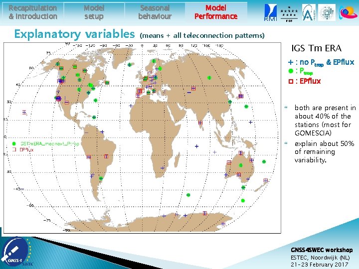
Recapitulation & introduction Model setup Explanatory variables Seasonal behaviour Model Performance ROB (means + all teleconnection patterns) IGS Tm ERA + : no Ptrop & EPflux ● : Ptrop □ : EPflux both are present in about 40% of the stations (most for GOMESCIA) explain about 50% of remaining variability. GNSS 4 SWEC workshop ESTEC, Noordwijk (NL) 21 -23 February 2017

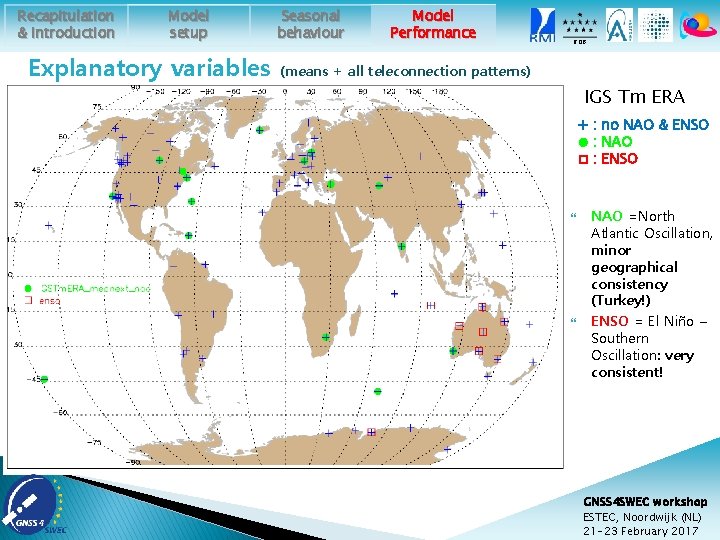
Recapitulation & introduction Model setup Explanatory variables Seasonal behaviour Model Performance ROB (means + all teleconnection patterns) IGS Tm ERA + : no NAO & ENSO ● : NAO □ : ENSO NAO =North Atlantic Oscillation, minor geographical consistency (Turkey!) ENSO = El Niño – Southern Oscillation: very consistent! GNSS 4 SWEC workshop ESTEC, Noordwijk (NL) 21 -23 February 2017

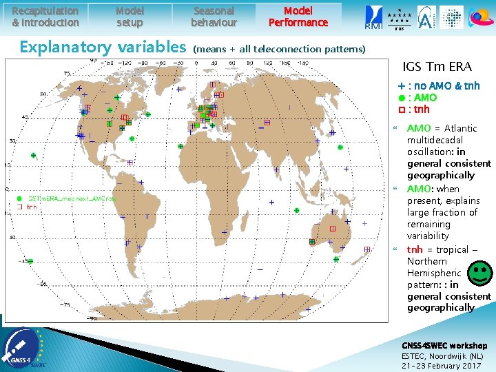
Recapitulation & introduction Model setup Explanatory variables Seasonal behaviour Model Performance ROB (means + all teleconnection patterns) IGS Tm ERA + : no AMO & tnh ● : AMO □ : tnh AMO = Atlantic multidecadal oscillation: in general consistent geographically AMO: when present, explains large fraction of remaining variability tnh = tropical – Northern Hemispheric pattern: : in general consistent geographically GNSS 4 SWEC workshop ESTEC, Noordwijk (NL) 21 -23 February 2017

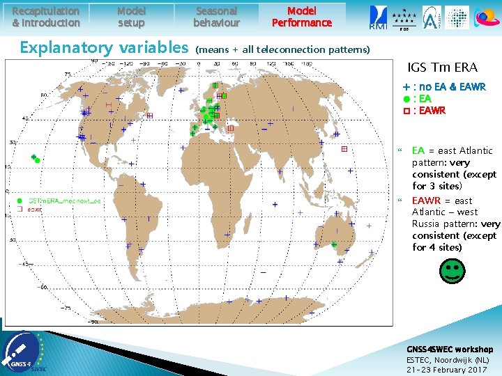
Recapitulation & introduction Model setup Explanatory variables Seasonal behaviour Model Performance ROB (means + all teleconnection patterns) IGS Tm ERA + : no EA & EAWR ● : EA □ : EAWR EA = east Atlantic pattern: very consistent (except for 3 sites) EAWR = east Atlantic – west Russia pattern: very consistent (except for 4 sites) GNSS 4 SWEC workshop ESTEC, Noordwijk (NL) 21 -23 February 2017

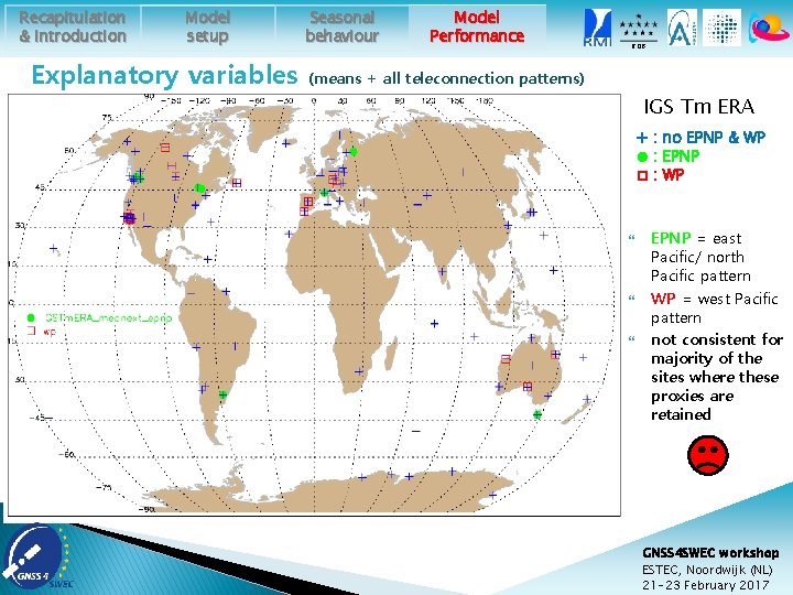
Recapitulation & introduction Model setup Explanatory variables Seasonal behaviour Model Performance ROB (means + all teleconnection patterns) IGS Tm ERA + : no EPNP & WP ● : EPNP □ : WP EPNP = east Pacific/ north Pacific pattern WP = west Pacific pattern not consistent for majority of the sites where these proxies are retained GNSS 4 SWEC workshop ESTEC, Noordwijk (NL) 21 -23 February 2017

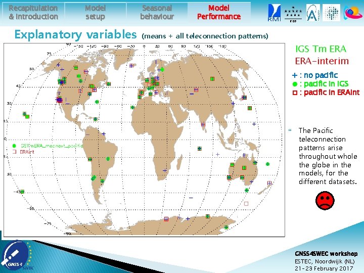
Recapitulation & introduction Model setup Explanatory variables Seasonal behaviour Model Performance ROB (means + all teleconnection patterns) IGS Tm ERA-interim + : no pacific ● : pacific in IGS □ : pacific in ERAint The Pacific teleconnection patterns arise throughout whole the globe in the models, for the different datasets. GNSS 4 SWEC workshop ESTEC, Noordwijk (NL) 21 -23 February 2017

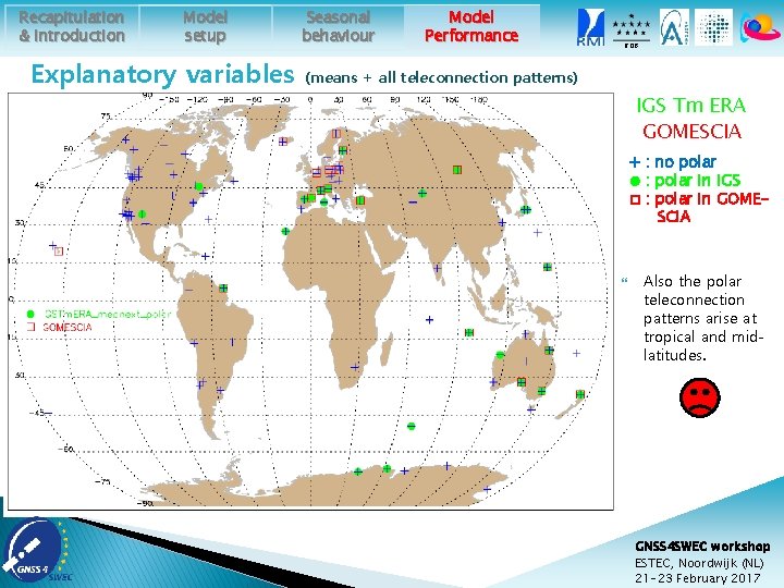
Recapitulation & introduction Model setup Explanatory variables Seasonal behaviour Model Performance ROB (means + all teleconnection patterns) IGS Tm ERA GOMESCIA + : no polar ● : polar in IGS □ : polar in GOMESCIA Also the polar teleconnection patterns arise at tropical and midlatitudes. GNSS 4 SWEC workshop ESTEC, Noordwijk (NL) 21 -23 February 2017

ROB Conclusions & Perspectives This simple, empirical model, works well for the NH mid-latitude sites (high correlation coefficients, geographically consistent proxies used). For other geographical regions (e. g. Australia, the Pacific), this approach is less successful (missing proxies? ) or all time series have more problems. The bulk of the variability is explained by the surface temperature (after accounting for the seasonal cycle by the long term means or the harmonics) long term variability (Claussius-Clapeyron) and/or remaining seasonality? A linear trend was retained as explanatory variable only for few sites. The residuals only show for a small number of sites significant trends, with the exception of GOMESCIA, where 20 to 30% show significant positive trends. So, there might be a clear homogenization issue in this dataset. future work: ◦ upgrade of the datasets used (ERA-interim 6 h & 18 h, GOMESCIA climate) ◦ monthly daily? ◦ publication in SI in prep. GNSS 4 SWEC workshop ESTEC, Noordwijk (NL) 21 -23 February 2017

painting by Jess Sutton Thank you! GNSS 4 SWEC workshop ESTEC, Noordwijk (NL) 21 -23 February 2017

Recapitulation & introduction Model setup Seasonal behaviour Model Performance ROB Teleconnection patterns recurring and persistent, large-scale patterns of pressure and circulation anomalies that spans vast geographical areas Although these patterns typically last for several weeks to several months, they can sometimes be prominent for several consecutive years, thus reflecting an important part of both the interannual and interdecadal variability of the atmospheric circulation. Many of the teleconnection patterns are also planetary-scale in nature, and span entire ocean basins and continents. a naturally occurring aspect of our chaotic atmospheric system, reflect large-scale changes in the atmospheric wave and jet stream patterns, and influence temperature, rainfall, storm tracks, and jet stream location/ intensity over vast areas seasonal weather forecast e. g. NAO = difference of atmospheric pressure at sea level between the Icelandic low and the Azores high. GNSS 4 SWEC workshop ESTEC, Noordwijk (NL) 21 -23 February 2017

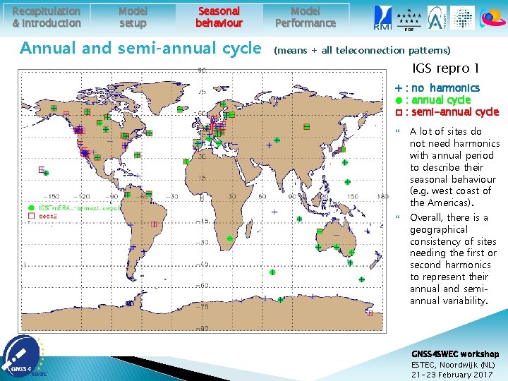
Recapitulation & introduction Model setup Seasonal behaviour Annual and semi-annual cycle Model Performance ROB (means + all teleconnection patterns) IGS repro 1 + : no harmonics ● : annual cycle □ : semi-annual cycle A lot of sites do not need harmonics with annual period to describe their seasonal behaviour (e. g. west coast of the Americas). Overall, there is a geographical consistency of sites needing the first or second harmonics to represent their annual and semiannual variability. GNSS 4 SWEC workshop ESTEC, Noordwijk (NL) 21 -23 February 2017