Route Prediction form Cellular Data KARI LAASONEN BASIC

Route Prediction form Cellular Data KARI LAASONEN BASIC RESEARCH UNIT, HELSINKI INSTITUTE FOR INFORMATION TECHNOLOGY DEPARTMENT OF COMPUTER SCIENCE, UNIVERSITY OF HELSINKI WORKSHOP ON CONTEXT-AWARENESS FOR PROACTIVE SYSTEMS 2005

Outline 2 1. Introduction 2. Problem Description 3. Prediction Algorithm 3. 1 Route Composition 3. 2 Route Similarity 3. 3 Making Predictions 4 Evaluation Comments

1. Introduction-1 3 Location awareness plays a large role in ubiquitous computing. Several applications relied on knowing or predicting the location of the user. Not merely to a known location, but to accurately predict human movement Early-reminder system Traffic planning We present an algorithm for predicting movement from cell-based location data. to learn places that are personally important to that user, To predict the place the user is moving to.

1. Introduction-2 4 Existing approaches to learning important locations and predicting routes rely on GPS data such as [4, 2] GPS can be problematic in urban areas Privacy. The contribution of the present paper an enhanced algorithm for predicting routes. The algorithm analyzes whole paths using string processing techniques, instead of relying on the short path fragments of the earlier paper. 2. Harrington, A. , Cahill, V. : Route Proling--Putting Context to Work. In: 2004 ACM Symposium on Applied Computing SAC'04, ACM Press(2004) 1567 -1573 4. Marmasse, N. , Schmandt, C. : A User-centered Location Model. Personal and Ubiquitous Computing 6 (2002) 318 -321

2 Problem Description 2. 1 Locations and Bases 5 Problem A GSM phone communicates with a base station. over the air several base stations signal reaches the phone. Select the station which has the strongest signal How about the signal strengths are equal? A cell is the area covered by a single base station we say the phone is in cell the phone is in the area of the corresponding base station. overlapping each other A physical location does not one-to-one to cells

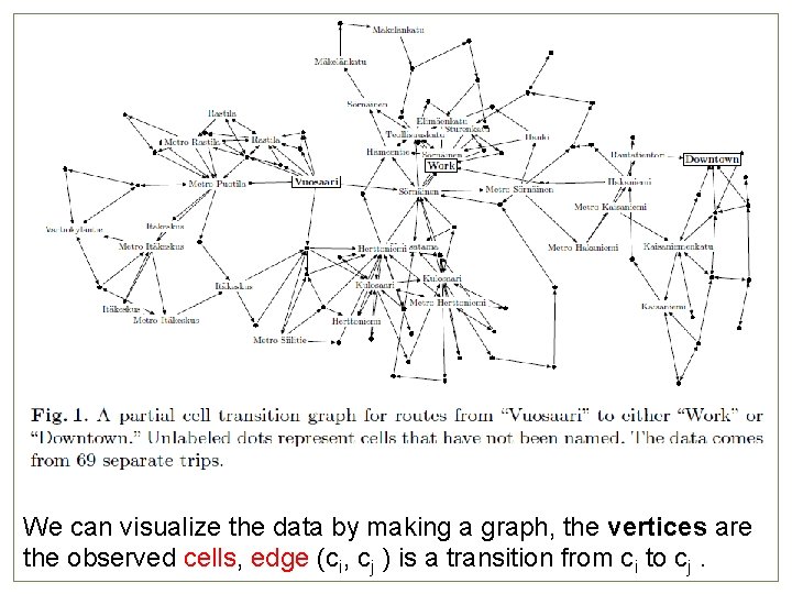
We can visualize the data by making a graph, the vertices are the observed cells, edge (ci, cj )6 is a transition from ci to cj.

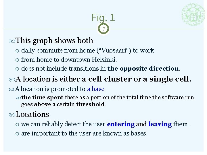
Fig. 1 7 This graph shows both daily commute from home (“Vuosaari”) to work from home to downtown Helsinki. does not include transitions in the opposite direction. A location is either a cell cluster or a single cell. A location is promoted to a base the time spent there as a portion of the total time the software run goes above a certain threshold. Locations we can reliably detect the user entering and leaving them. are important to the user are known as bases.

2. 2 Route Prediction 8 the most important consequence of using cell- based location data is that lack the physical topology of the cell network. includes the correspondence between cells and physical locations, and also all indications of direction. cell sequence: ABA? the user visited B and came back. Or cell A was just briefly shadowed by B. Looking at the immediate context is all but useless.

Two basic approaches to the problem-1 9 The first is to examine the local context of recent cells [3]. Suppose in cell c and the have been h 1, h 2… prepare strings hkhk-1 …h 1 c, variable k. matched against a database of stored fragments. Based on the matches found, and the bases reached from c, we get probabilities for the next base. 3. Laasonen, K. , Raento, M. , Toivonen, H. : Adaptive On-device Location Recognition. In Pervasive Computing: Second International Conference, LNCS 3001, Springer Verlag (2004), 287{304

Two basic approaches to the problem-2 10 The second approach, in this paper entire routes between two bases. To learn all different physical routes as strings of cell identifiers. Whenever the user completes a route r between bases a and b if an existing route between a and b is similar to r. the two routes are merged together. To make a prediction the user has left base a, we have a set of possible routes and their destinations b. We now use a recent history h of cells and find the route that exhibits the largest similarity to h.

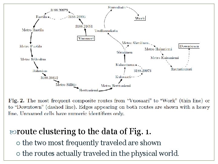
route clustering to the data of Fig. 1. the two most frequently traveled are shown the routes actually traveled in the physical world. 11

3. Prediction Algorithm 12 There are three phases in the algorithm. Phase 1, the user leaves a base enters a cell c, prepares for a new route prediction task. Phase 2, at each cell transition, we make a prediction, which is a set of pairs (b, p), b is a possible future base p the probability of the user going Phase 3, when the user arrives at a base, the entire route a, c 1, …, cn, b* is used to make better subsequent predictions.

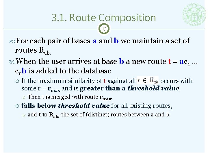
3. 1. Route Composition 13 For each pair of bases a and b we maintain a set of routes Rab. When the user arrives at base b a new route t = ac 1 … cnb is added to the database If the maximum similarity of t against all occurs with some r = rmax and is greater than a threshold value. Then t is merged with route rmax. falls below threshold value for all existing routes, add t to Rab, the set of (distinct) routes between a and b.

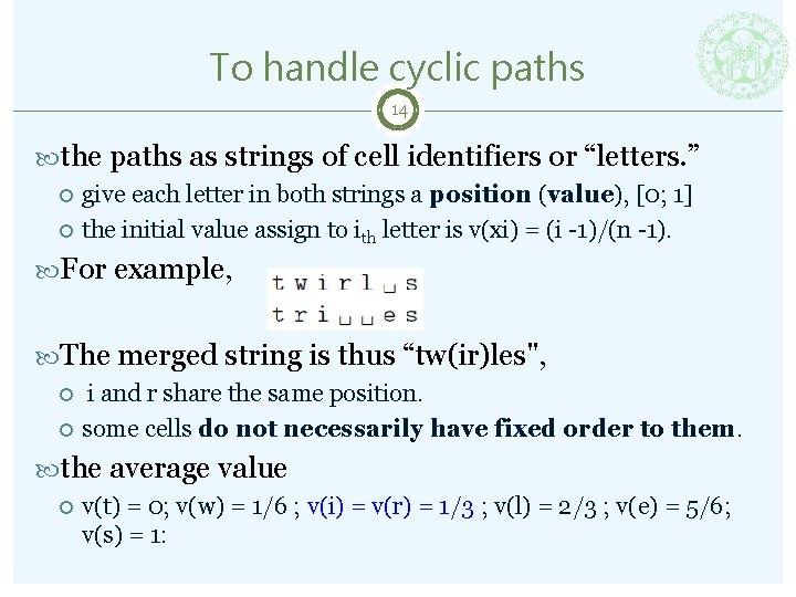
To handle cyclic paths 14 the paths as strings of cell identifiers or “letters. ” give each letter in both strings a position (value), [0; 1] the initial value assign to ith letter is v(xi) = (i -1)/(n -1). For example, The merged string is thus “tw(ir)les", i and r share the same position. some cells do not necessarily have fixed order to them. the average value v(t) = 0; v(w) = 1/6 ; v(i) = v(r) = 1/3 ; v(l) = 2/3 ; v(e) = 5/6; v(s) = 1:

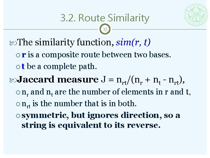
3. 2. Route Similarity 15 The similarity function, sim(r, t) r is a composite route between two bases. t be a complete path. Jaccard measure J = nrt/(nr + nt - nrt), nr and nt are the number of elements in r and t, nrt is the number that is in both. symmetric, but ignores direction, so a string is equivalent to its reverse.

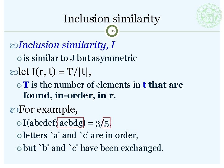
Inclusion similarity 16 Inclusion similarity, I is similar to J but asymmetric let I(r, t) = T/|t|, T is the number of elements in t that are found, in-order, in r. For example, I(abcdef; acbdg) = 3/5; letters `a' and `c' are in order, but `b' and `c' have been exchanged.

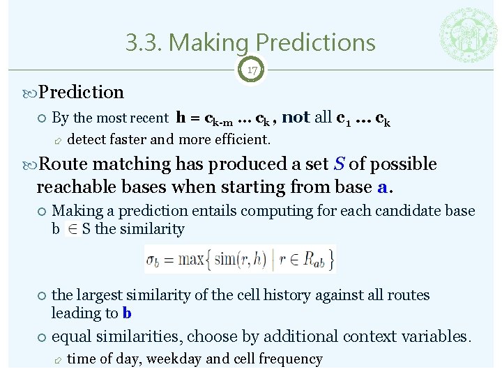
3. 3. Making Predictions 17 Prediction By the most recent h = ck-m … ck , not all c 1 … ck detect faster and more efficient. Route matching has produced a set S of possible reachable bases when starting from base a. Making a prediction entails computing for each candidate base b S the similarity the largest similarity of the cell history against all routes leading to b equal similarities, choose by additional context variables. time of day, weekday and cell frequency

4. Evaluation 18 The data was collected for six months in 2003 With the Context Phone software on a Nokia 7650 phone. three volunteer users both at work and at leisure. The baseline algorithm is the fragment-based method [3], which was tested with several window sizes k. The resulting prediction was then compared to the actual base. 3. Laasonen, K. , Raento, M. , Toivonen, H. : Adaptive On-device Location Recognition. In Pervasive Computing: Second International Conference, LNCS 3001, Springer Verlag (2004), 287{304

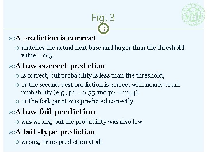
Fig. 3 19 A prediction is correct matches the actual next base and larger than the threshold value = 0. 3. A low correct prediction is correct, but probability is less than the threshold, or the second-best prediction is correct with nearly equal probability (e. g. , p 1 = 0: 55 and p 2 = 0: 44), or the fork point was predicted correctly. A low fail prediction was wrong, but the probability was also low. A fail -type prediction wrong, or no prediction at all.

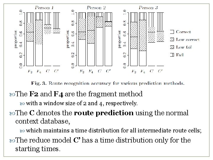
The F 2 and F 4 are the fragment method with a window size of 2 and 4, respectively. The C denotes the route prediction using the normal context database, which maintains a time distribution for all intermediate route cells; The reduce model C’ has a time distribution only for the starting times. 20

Fig. 4 21 Accuracy models C and C’ are very similar the latter uses much less memory But even model C Fig. 4 Comparison of the memory consumption of the algorithms. consumes less memory than any fragment-based method.

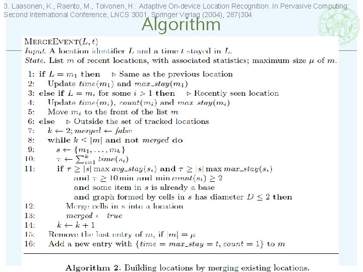
3. Laasonen, K. , Raento, M. , Toivonen, H. : Adaptive On-device Location Recognition. In Pervasive Computing: Second International Conference, LNCS 3001, Springer Verlag (2004), 287{304 Algorithm 23