ROOT Tutorial Simulation and fitting in ROOT Attilio

ROOT Tutorial Simulation and fitting in ROOT Attilio Andreazza Università di Milano and INFN Caterina Doglioni Université de Genève

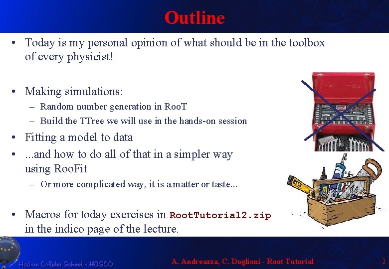
Outline • Today is my personal opinion of what should be in the toolbox of every physicist! • Making simulations: – Random number generation in Roo. T – Build the TTree we will use in the hands-on session • Fitting a model to data • . . . and how to do all of that in a simpler way using Roo. Fit – Or more complicated way, it is a matter or taste. . . • Macros for today exercises in Root. Tutorial 2. zip in the indico page of the lecture. A. Andreazza, C. Doglioni - Root Tutorial 2

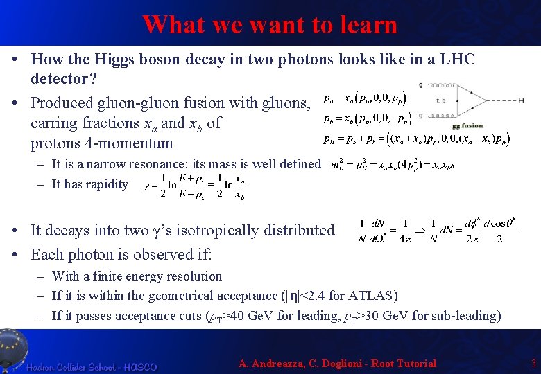
What we want to learn • How the Higgs boson decay in two photons looks like in a LHC detector? • Produced gluon-gluon fusion with gluons, carring fractions xa and xb of protons 4 -momentum – It is a narrow resonance: its mass is well defined – It has rapidity • It decays into two g’s isotropically distributed • Each photon is observed if: – With a finite energy resolution – If it is within the geometrical acceptance (|h|<2. 4 for ATLAS) – If it passes acceptance cuts (p. T>40 Ge. V for leading, p. T>30 Ge. V for sub-leading) A. Andreazza, C. Doglioni - Root Tutorial 3

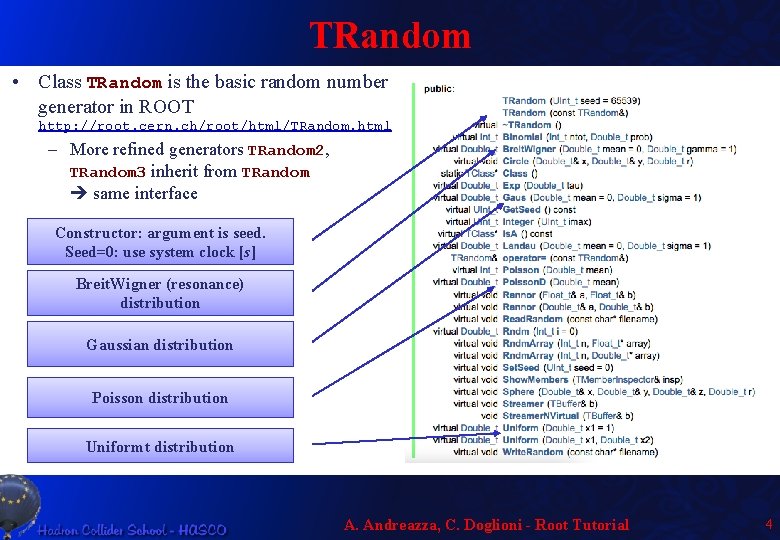
TRandom • Class TRandom is the basic random number generator in ROOT http: //root. cern. ch/root/html/TRandom. html – More refined generators TRandom 2, TRandom 3 inherit from TRandom same interface Constructor: argument is seed. Seed=0: use system clock [s] Breit. Wigner (resonance) distribution Gaussian distribution Poisson distribution Uniformt distribution A. Andreazza, C. Doglioni - Root Tutorial 4

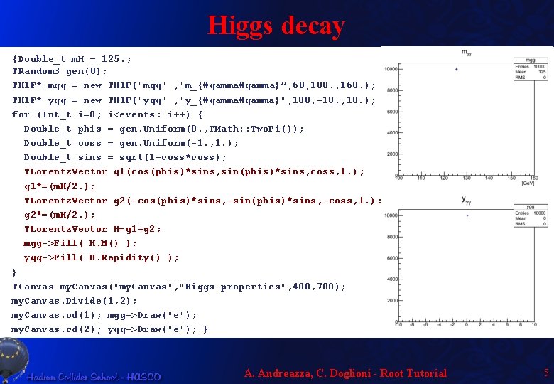
Higgs decay {Double_t m. H = 125. ; TRandom 3 gen(0); TH 1 F* mgg = new TH 1 F("mgg" , "m_{#gamma}”, 60, 100. , 160. ); TH 1 F* ygg = new TH 1 F("ygg" , "y_{#gamma}", 100, -10. , 10. ); for (Int_t i=0; i<events; i++) { Double_t phis = gen. Uniform(0. , TMath: : Two. Pi()); Double_t coss = gen. Uniform(-1. , 1. ); Double_t sins = sqrt(1 -coss*coss); TLorentz. Vector g 1(cos(phis)*sins, sin(phis)*sins, coss, 1. ); g 1*=(m. H/2. ); TLorentz. Vector g 2(-cos(phis)*sins, -sin(phis)*sins, -coss, 1. ); g 2*=(m. H/2. ); TLorentz. Vector H=g 1+g 2; mgg->Fill( H. M() ); ygg->Fill( H. Rapidity() ); } TCanvas my. Canvas("my. Canvas", "Higgs properties", 400, 700); my. Canvas. Divide(1, 2); my. Canvas. cd(1); mgg->Draw("e"); my. Canvas. cd(2); ygg->Draw("e"); } A. Andreazza, C. Doglioni - Root Tutorial 5

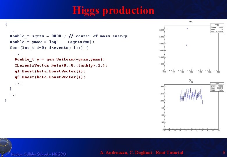
Higgs production {. . . Double_t sqrts = 8000. ; // center of mass energy Double_t ymax = log (sqrts/m. H); for (Int_t i=0; i<events; i++) {. . . Double_t y = gen. Uniform(-ymax, ymax); TLorentz. Vector beta(0. , tanh(y), 1. ); g 1. Boost(beta. Boost. Vector()); g 2. Boost(beta. Boost. Vector()); . . . } A. Andreazza, C. Doglioni - Root Tutorial 6

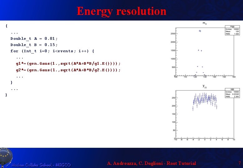
Energy resolution {. . . Double_t A = 0. 01; Double_t B = 0. 15; for (Int_t i=0; i<events; i++) {. . . g 1*=(gen. Gaus(1. , sqrt(A*A+B*B/g 1. E()))); g 2*=(gen. Gaus(1. , sqrt(A*A+B*B/g 2. E()))); . . . } A. Andreazza, C. Doglioni - Root Tutorial 7

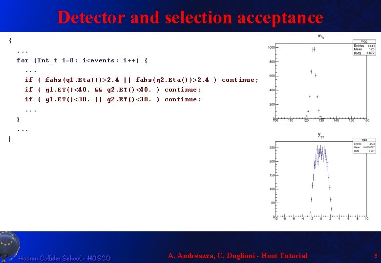
Detector and selection acceptance {. . . for (Int_t i=0; i<events; i++) {. . . if ( fabs(g 1. Eta())>2. 4 || fabs(g 2. Eta())>2. 4 ) continue; if ( g 1. ET()<40. && g 2. ET()<40. ) continue; if ( g 1. ET()<30. || g 2. ET()<30. ) continue; . . . } A. Andreazza, C. Doglioni - Root Tutorial 8

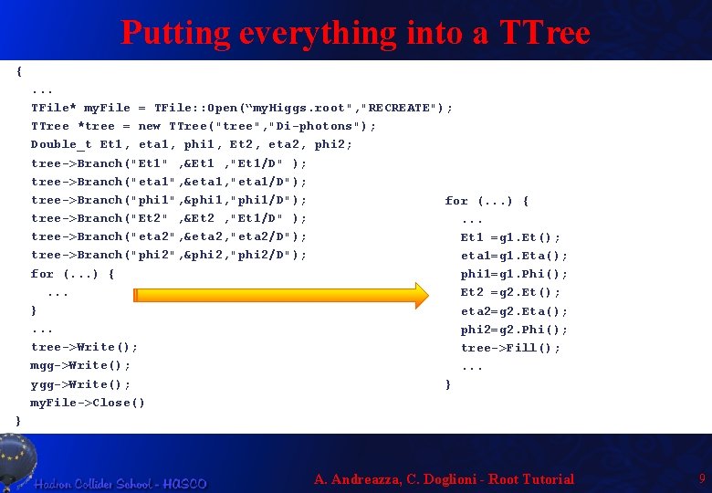
Putting everything into a TTree {. . . TFile* my. File = TFile: : Open(“my. Higgs. root", "RECREATE"); TTree *tree = new TTree("tree", "Di-photons"); Double_t Et 1, eta 1, phi 1, Et 2, eta 2, phi 2; tree->Branch("Et 1" , &Et 1 , "Et 1/D" ); tree->Branch("eta 1", &eta 1, "eta 1/D"); tree->Branch("phi 1", &phi 1, "phi 1/D"); for (. . . ) { tree->Branch("Et 2" , &Et 2 , "Et 1/D" ); . . . tree->Branch("eta 2", &eta 2, "eta 2/D"); Et 1 =g 1. Et(); tree->Branch("phi 2", &phi 2, "phi 2/D"); eta 1=g 1. Eta(); for (. . . ) { phi 1=g 1. Phi(); . . . Et 2 =g 2. Et(); } eta 2=g 2. Eta(); . . . phi 2=g 2. Phi(); tree->Write(); tree->Fill(); mgg->Write(); . . . ygg->Write(); } my. File->Close() } A. Andreazza, C. Doglioni - Root Tutorial 9

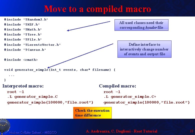
Move to a compiled macro #include #include "TRandom 3. h" "TH 1 F. h" "TMath. h" "TTree. h" "TFile. h" "TLorentz. Vector. h" "TCanvas. h" All used classes need their corresponding header file Define interface to interactively change number of events and output file #include <cmath> void generator_simple(Int_t events, char* filename) {. . . } Interpreted macro: Compiled macro: root –l. L generator_simple. C generator_simple(100000, ”file. root”) root –l. L generator_simple. C+ generator_simple(100000, ”file. root”) Check the execution time difference A. Andreazza, C. Doglioni - Root Tutorial 10

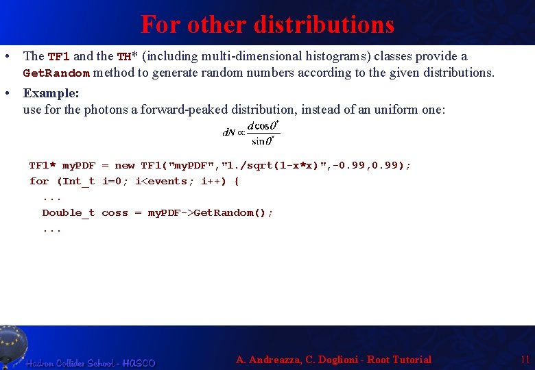
For other distributions • The TF 1 and the TH* (including multi-dimensional histograms) classes provide a Get. Random method to generate random numbers according to the given distributions. • Example: use for the photons a forward-peaked distribution, instead of an uniform one: TF 1* my. PDF = new TF 1("my. PDF", "1. /sqrt(1 -x*x)", -0. 99, 0. 99); for (Int_t i=0; i<events; i++) {. . . Double_t coss = my. PDF->Get. Random(); . . . A. Andreazza, C. Doglioni - Root Tutorial 11

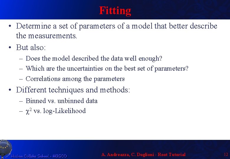
Fitting • Determine a set of parameters of a model that better describe the measurements. • But also: – Does the model described the data well enough? – Which are the uncertainties on the best set of parameters? – Correlations among the parameters • Different techniques and methods: – Binned vs. unbinned data – c 2 vs. log-Likelihood A. Andreazza, C. Doglioni - Root Tutorial 12

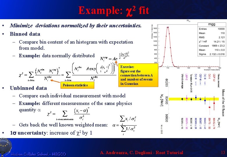
Example: c 2 fit • Minimize deviations normalized by their uncertainties. • Binned data – Compare bin content of an histogram with expectation from model. – Example: data normally distributed • Unbinned data Exercise: figure out the connection between A and number of events in Gaussian Poisson statistics – Compare each individual measurement with model – Example: different measuremens of the same physics quantity a – Gets back the well known weighted mean: • 1 s uncertainty: increase of c 2 by 1 A. Andreazza, C. Doglioni - Root Tutorial 13

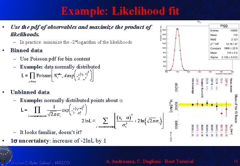
Example: Likelihood fit • Use the pdf of observables and maximize the product of likelihoods. – In practice: minimize the -2*logarithm of the likelihoods • Binned data – Use Poisson pdf for bin content – Example: data normally distributed • Unbinned data – Example: normally distributed points about a – It looks familiar, doesn’t it? • 1 s uncertainty: increase of -2 ln. L by 1 A. Andreazza, C. Doglioni - Root Tutorial 14

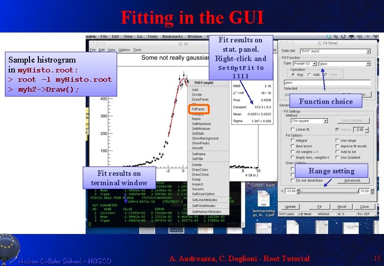
Fitting in the GUI Fit results on stat. panel. Right-click and Set. Opt. Fit to Sample histrogram in my. Histo. root: > root –l my. Histo. root > myh 2 ->Draw(); 1111 Function choice Fit results on terminal window Range setting A. Andreazza, C. Doglioni - Root Tutorial 15

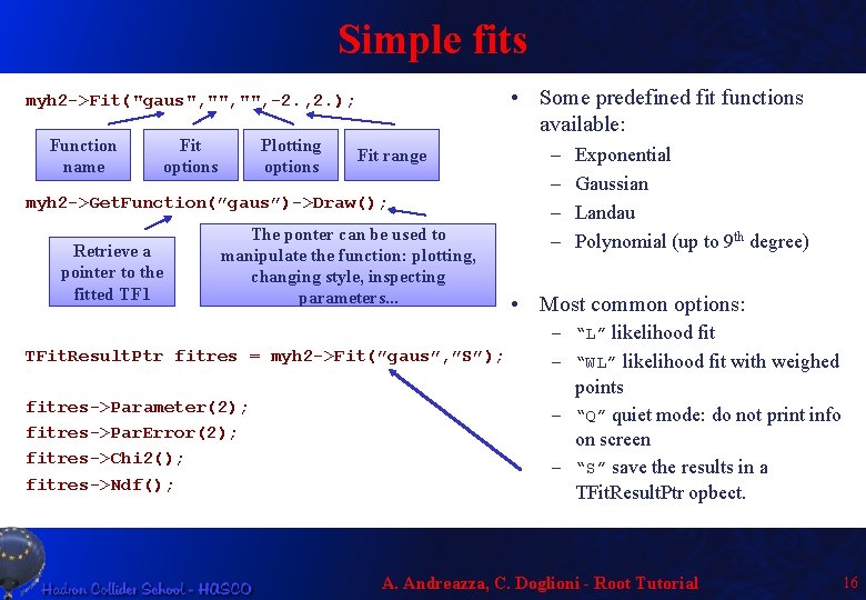
Simple fits • Some predefined fit functions available: myh 2 ->Fit("gaus", "", -2. , 2. ); Function name Fit options Plotting options Fit range myh 2 ->Get. Function(”gaus”)->Draw(); Retrieve a pointer to the fitted TF 1 The ponter can be used to manipulate the function: plotting, changing style, inspecting parameters. . . – – Exponential Gaussian Landau Polynomial (up to 9 th degree) • Most common options: – “L” likelihood fit TFit. Result. Ptr fitres = myh 2 ->Fit(”gaus”, ”S”); – “WL” likelihood fit with weighed fitres->Parameter(2); fitres->Par. Error(2); fitres->Chi 2(); fitres->Ndf(); points – “Q” quiet mode: do not print info on screen – “S” save the results in a TFit. Result. Ptr opbect. A. Andreazza, C. Doglioni - Root Tutorial 16

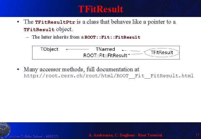
TFit. Result • The TFit. Result. Ptr is a class that behaves like a pointer to a TFit. Result object. – The latter inherits from a ROOT: : Fit. Result • Many accessor methods, full documentation at http: //root. cern. ch/root/html/ROOT__Fit. Result. html A. Andreazza, C. Doglioni - Root Tutorial 17

TFit. Result root [38] TFit. Result. Ptr fitres = myh 2 ->Fit("gaus", "S", "", -2. , 2. ) FCN=16. 5644 FROM MIGRAD STATUS=CONVERGED 71 CALLS 72 TOTAL EDM=6. 18403 e-09 STRATEGY= 1 ERROR MATRIX ACCURATE EXT PARAMETER STEP FIRST NO. NAME VALUE ERROR SIZE DERIVATIVE 1 Constant 5. 12179 e+02 8. 19111 e+00 1. 21137 e-02 2. 10983 e-06 2 Mean -1. 99953 e-02 2. 13804 e-02 4. 36950 e-05 -5. 06752 e-03 3 Sigma 1. 35596 e+00 2. 78382 e-02 1. 20495 e-05 -1. 87226 e-03 root [39] fitres->Print(cout) ******************** Minimizer is Minuit / Migrad Chi 2 = 16. 5644 NDf = 17 Edm = 6. 18403 e-09 NCalls = 72 Constant = 512. 179 Mean = -0. 0199953 Sigma = 1. 35596 +/+/+/- 8. 19111 0. 0213804 0. 0278382 (limited) A. Andreazza, C. Doglioni - Root Tutorial 18

TFit. Result root [40] fitres->Print. Cov. Matrix(cout) Covariance Matrix: Constant Mean Sigma 67. 094 0. 0048267 -0. 1576 0. 0048267 0. 00045712 -2. 9505 e-05 -0. 1576 -2. 9505 e-05 0. 00077498 Correlation Matrix: Constant Mean Sigma root [41] Constant 1 0. 027561 -0. 69116 Mean 0. 027561 1 -0. 049571 Sigma -0. 69116 -0. 049571 1 A. Andreazza, C. Doglioni - Root Tutorial 19

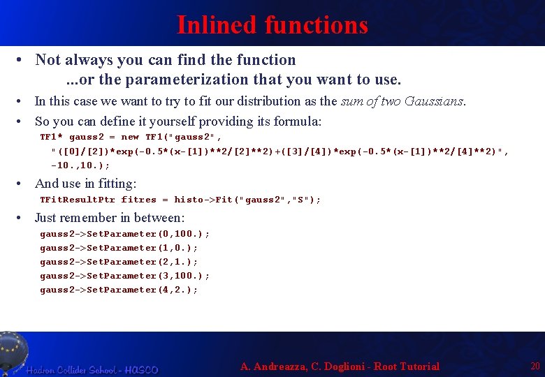
Inlined functions • Not always you can find the function. . . or the parameterization that you want to use. • In this case we want to try to fit our distribution as the sum of two Gaussians. • So you can define it yourself providing its formula: TF 1* gauss 2 = new TF 1("gauss 2", "([0]/[2])*exp(-0. 5*(x-[1])**2/[2]**2)+([3]/[4])*exp(-0. 5*(x-[1])**2/[4]**2)", -10. , 10. ); • And use in fitting: TFit. Result. Ptr fitres = histo->Fit("gauss 2", "S"); • Just remember in between: gauss 2 ->Set. Parameter(0, 100. ); gauss 2 ->Set. Parameter(1, 0. ); gauss 2 ->Set. Parameter(2, 1. ); gauss 2 ->Set. Parameter(3, 100. ); gauss 2 ->Set. Parameter(4, 2. ); A. Andreazza, C. Doglioni - Root Tutorial 20

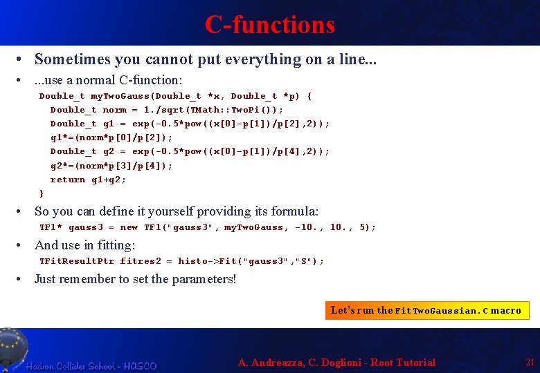
C-functions • Sometimes you cannot put everything on a line. . . • . . . use a normal C-function: Double_t my. Two. Gauss(Double_t *x, Double_t *p) { Double_t norm = 1. /sqrt(TMath: : Two. Pi()); Double_t g 1 = exp(-0. 5*pow((x[0]-p[1])/p[2], 2)); g 1*=(norm*p[0]/p[2]); Double_t g 2 = exp(-0. 5*pow((x[0]-p[1])/p[4], 2)); g 2*=(norm*p[3]/p[4]); return g 1+g 2; } • So you can define it yourself providing its formula: TF 1* gauss 3 = new TF 1("gauss 3", my. Two. Gauss, -10. , 5); • And use in fitting: TFit. Result. Ptr fitres 2 = histo->Fit("gauss 3", "S"); • Just remember to set the parameters! Let’s run the Fit. Two. Gaussian. C macro A. Andreazza, C. Doglioni - Root Tutorial 21

. . . and when things starts to become really complicated ROOFIT

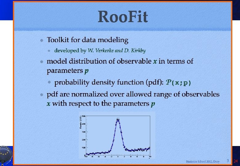
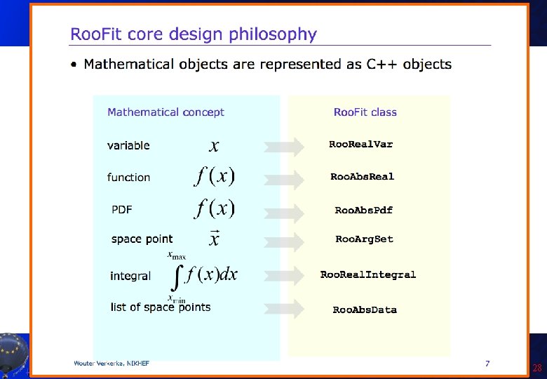
Introduction to Roo. Fit • Disclaimer: I am not a Roo. Fit expert: I learnt it last week because of you! Only few of the features will be presented here! • So you can get much better material from the official sources: – Roo. Fit web page: http: //roofit. sourceforge. net/ – Roo. Fit tutorials: http: //root. cern. ch/root/html/tutorials/roofit/index. html – Roo. Fit entry in the ROOT reference guide: http: //root. cern. ch/root/html/ROOFIT_Index. html • In particular I appreciated a lot the tutorial at the Desy 2012 School of Statistics by L. Moneta and S. Kreiss: https: //twiki. cern. ch/twiki/bin/view/Roo. Stats/Web. Home#Resources many slides here by them and W. Werverke A. Andreazza, C. Doglioni - Root Tutorial 23

A. Andreazza, C. Doglioni - Root Tutorial 24

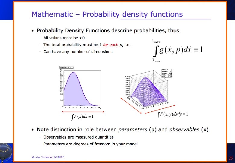
A. Andreazza, C. Doglioni - Root Tutorial 25

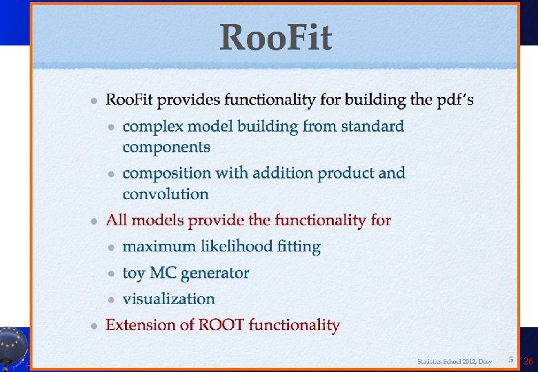
A. Andreazza, C. Doglioni - Root Tutorial 26

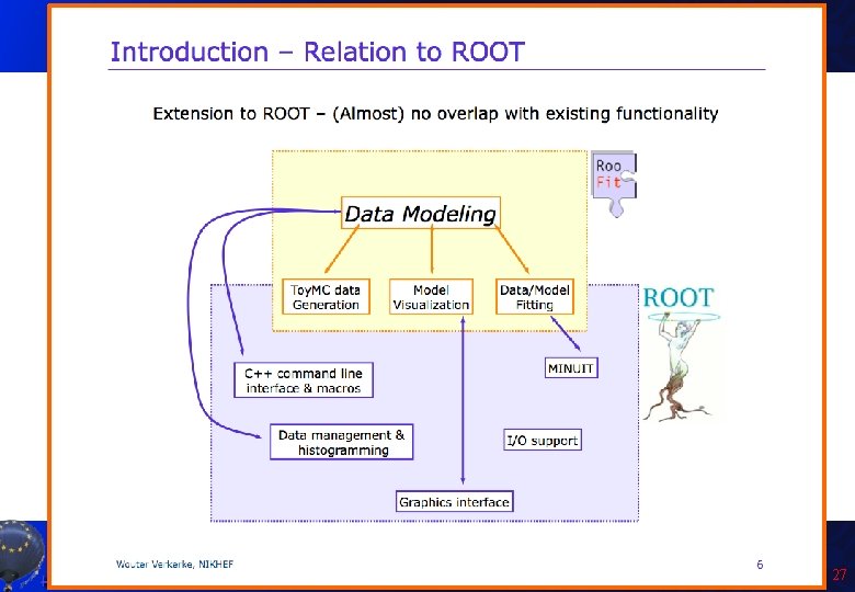
A. Andreazza, C. Doglioni - Root Tutorial 27

A. Andreazza, C. Doglioni - Root Tutorial 28

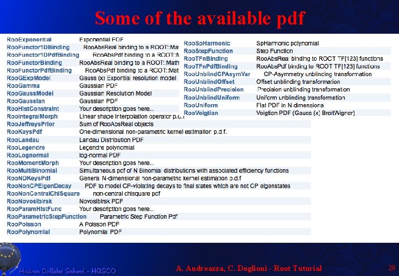
Some of the available pdf A. Andreazza, C. Doglioni - Root Tutorial 29

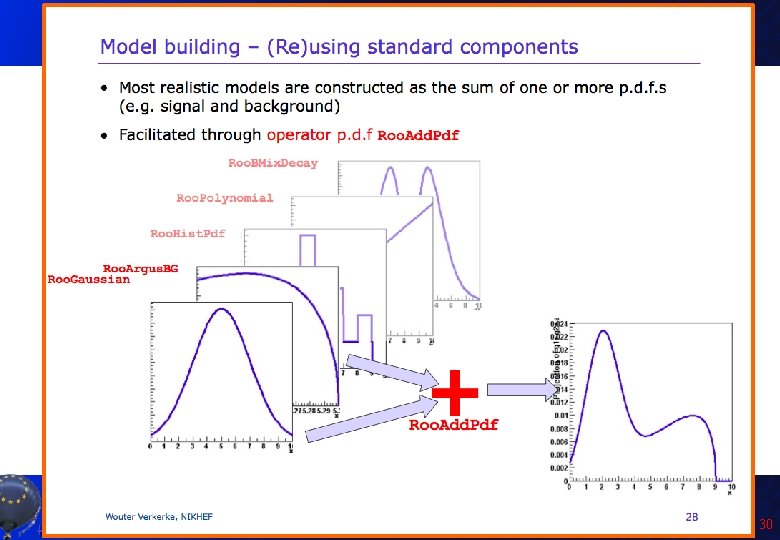
A. Andreazza, C. Doglioni - Root Tutorial 30

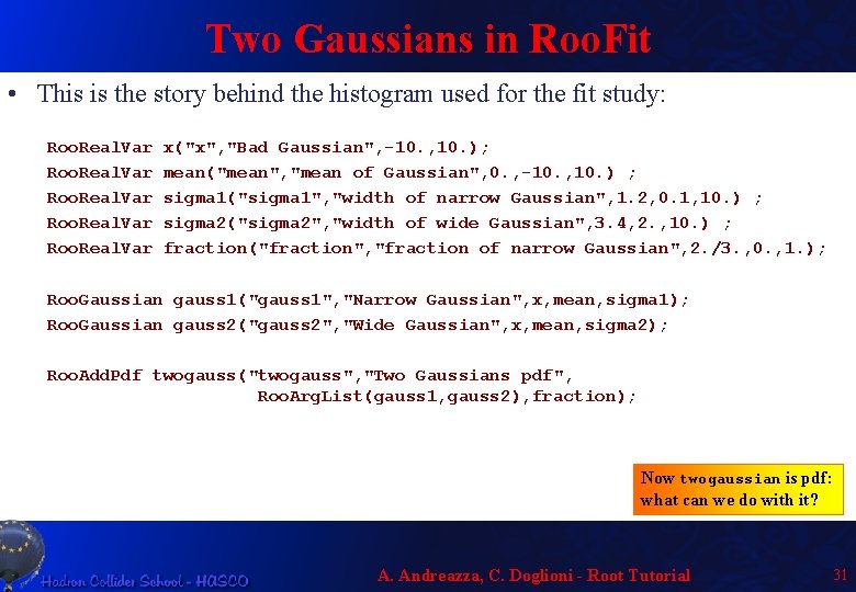
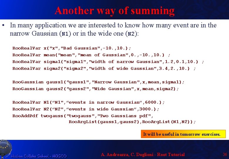
Two Gaussians in Roo. Fit • This is the story behind the histogram used for the fit study: Roo. Real. Var x("x", "Bad Gaussian", -10. , 10. ); mean("mean", "mean of Gaussian", 0. , -10. , 10. ) ; sigma 1("sigma 1", "width of narrow Gaussian", 1. 2, 0. 1, 10. ) ; sigma 2("sigma 2", "width of wide Gaussian", 3. 4, 2. , 10. ) ; fraction("fraction", "fraction of narrow Gaussian", 2. /3. , 0. , 1. ); Roo. Gaussian gauss 1("gauss 1", "Narrow Gaussian", x, mean, sigma 1); Roo. Gaussian gauss 2("gauss 2", "Wide Gaussian", x, mean, sigma 2); Roo. Add. Pdf twogauss("twogauss", "Two Gaussians pdf", Roo. Arg. List(gauss 1, gauss 2), fraction); Now twogaussian is pdf: what can we do with it? A. Andreazza, C. Doglioni - Root Tutorial 31

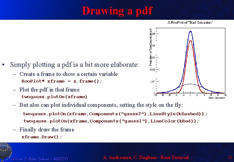
Drawing a pdf • Simply plotting a pdf is a bit more elaborate: – Create a frame to show a certain variable Roo. Plot* xframe = x. frame(); – Plot the pdf in that frame twogauss. plot. On(xframe) – But also can plot individual components, setting the style on the fly: twogauss. plot. On(xframe, Components("gauss 2"), Line. Style(k. Dashed)); twogauss. plot. On(xframe, Components("gauss 1"), Line. Color(k. Red)); – Finally draw the frame xframe. Draw(); A. Andreazza, C. Doglioni - Root Tutorial 32

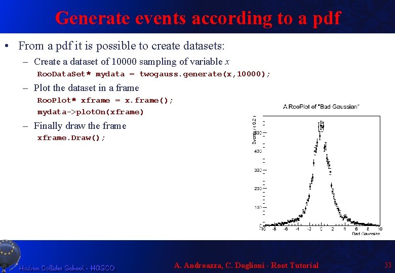
Generate events according to a pdf • From a pdf it is possible to create datasets: – Create a dataset of 10000 sampling of variable x Roo. Data. Set* mydata = twogauss. generate(x, 10000); – Plot the dataset in a frame Roo. Plot* xframe = x. frame(); mydata->plot. On(xframe) – Finally draw the frame xframe. Draw(); A. Andreazza, C. Doglioni - Root Tutorial 33

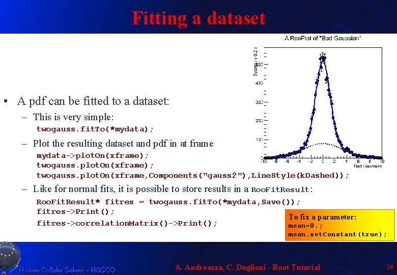
Fitting a dataset • A pdf can be fitted to a dataset: – This is very simple: twogauss. fit. To(*mydata); – Plot the resulting dataset and pdf in at frame mydata->plot. On(xframe); twogauss. plot. On(xframe, Components("gauss 2"), Line. Style(k. Dashed)); – Like for normal fits, it is possible to store results in a Roo. Fit. Result: Roo. Fit. Result* fitres = twogauss. fit. To(*mydata, Save()); fitres->Print(); To fix a parameter: fitres->correlation. Matrix()->Print(); mean=0. ; mean. set. Constant(true); A. Andreazza, C. Doglioni - Root Tutorial 34

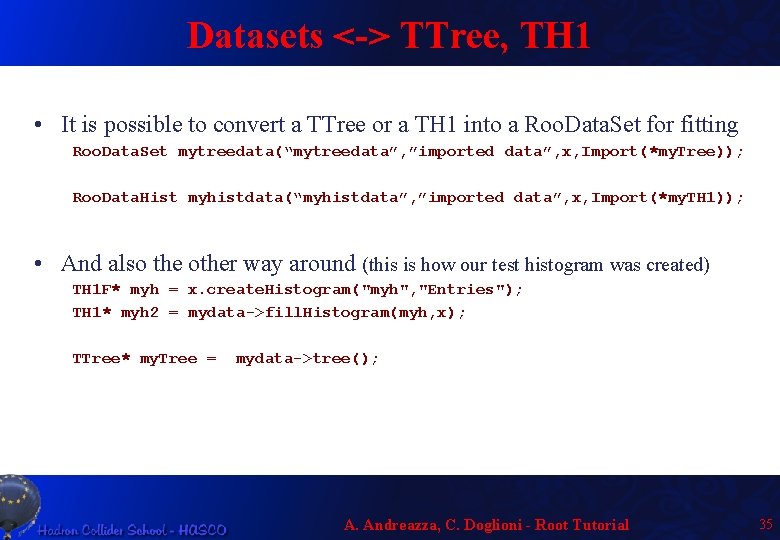
Datasets <-> TTree, TH 1 • It is possible to convert a TTree or a TH 1 into a Roo. Data. Set for fitting Roo. Data. Set mytreedata(“mytreedata”, ”imported data”, x, Import(*my. Tree)); Roo. Data. Hist myhistdata(“myhistdata”, ”imported data”, x, Import(*my. TH 1)); • And also the other way around (this is how our test histogram was created) TH 1 F* myh = x. create. Histogram("myh", "Entries"); TH 1* myh 2 = mydata->fill. Histogram(myh, x); TTree* my. Tree = mydata->tree(); A. Andreazza, C. Doglioni - Root Tutorial 35

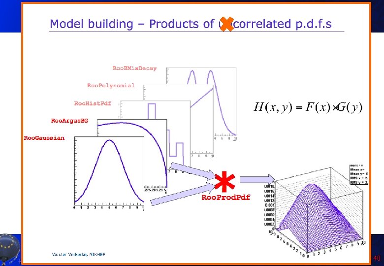
Another way of summing • In many application we are interested to know how many event are in the narrow Gaussian (N 1) or in the wide one (N 2): Roo. Real. Var x("x", "Bad Gaussian", -10. , 10. ); mean("mean", "mean of Gaussian", 0. , -10. , 10. ) ; sigma 1("sigma 1", "width of narrow Gaussian", 1. 2, 0. 1, 10. ) ; sigma 2("sigma 2", "width of wide Gaussian", 3. 4, 2. , 10. ) ; Roo. Gaussian gauss 1("gauss 1", "Narrow Gaussian", x, mean, sigma 1); Roo. Gaussian gauss 2("gauss 2", "Wide Gaussian", x, mean, sigma 2); Roo. Real. Var N 1(”N 1", ”events in narrow Gaussian”, 6000. ); Roo. Real. Var N 2(”N 2", ”events in wide Gaussian”, 3000. ); Roo. Add. Pdf twogauss("twogauss", "Two Gaussians pdf", Roo. Arg. List(gauss 1, gauss 2), Roo. Arg. List(N 1, N 2)); It will be useful in tomorrow exercises. A. Andreazza, C. Doglioni - Root Tutorial 36

A. Andreazza, C. Doglioni - Root Tutorial 37

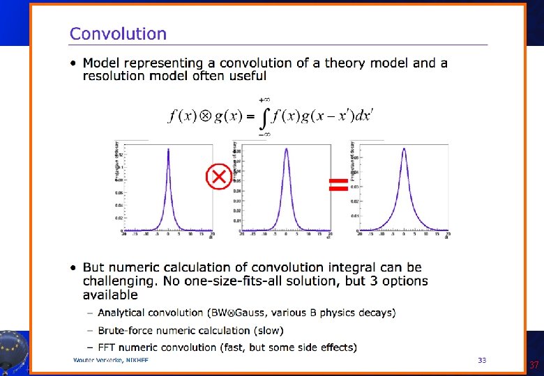
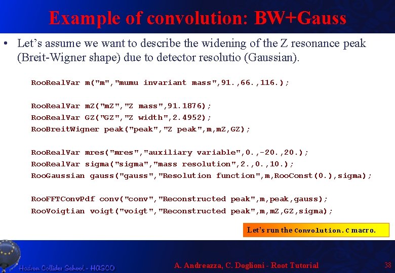
Example of convolution: BW+Gauss • Let’s assume we want to describe the widening of the Z resonance peak (Breit-Wigner shape) due to detector resolutio (Gaussian). Roo. Real. Var m("m", "mumu invariant mass", 91. , 66. , 116. ); Roo. Real. Var m. Z("m. Z", "Z mass", 91. 1876); Roo. Real. Var GZ("GZ", "Z width", 2. 4952); Roo. Breit. Wigner peak("peak", "Z peak", m, m. Z, GZ); Roo. Real. Var mres("mres", "auxiliary variable", 0. , -20. , 20. ); Roo. Real. Var sigma("sigma", "mass resolution", 2. , 0. , 10. ); Roo. Gaussian gauss("gauss", "Resolution function", m, Roo. Const(0. ), sigma); Roo. FFTConv. Pdf conv("conv", "Reconstructed peak", m, peak, gauss); Roo. Voigtian voigt("voigt", "Reconstructed peak", m, m. Z, GZ, sigma); Let’s run the Convolution. C macro. A. Andreazza, C. Doglioni - Root Tutorial 38

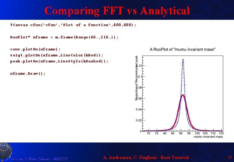
Comparing FFT vs Analytical TCanvas cfun("cfun", "Plot of a function", 400); Roo. Plot* xframe = m. frame(Range(66. , 116. )); conv. plot. On(xframe); voigt. plot. On(xframe, Line. Color(k. Red)); peak. plot. On(xframe, Line. Style(k. Dashed)); xframe. Draw(); A. Andreazza, C. Doglioni - Root Tutorial 39

A. Andreazza, C. Doglioni - Root Tutorial 40

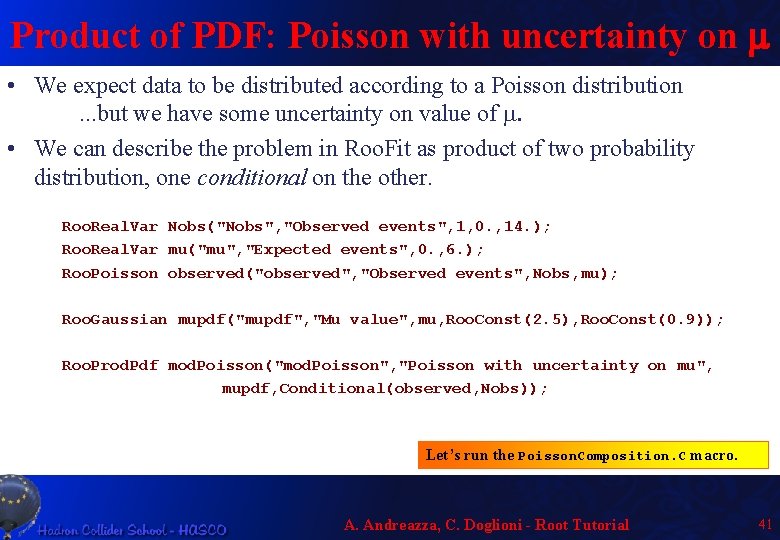
Product of PDF: Poisson with uncertainty on m • We expect data to be distributed according to a Poisson distribution. . . but we have some uncertainty on value of m. • We can describe the problem in Roo. Fit as product of two probability distribution, one conditional on the other. Roo. Real. Var Nobs("Nobs", "Observed events", 1, 0. , 14. ); Roo. Real. Var mu("mu", "Expected events", 0. , 6. ); Roo. Poisson observed("observed", "Observed events", Nobs, mu); Roo. Gaussian mupdf("mupdf", "Mu value", mu, Roo. Const(2. 5), Roo. Const(0. 9)); Roo. Prod. Pdf mod. Poisson("mod. Poisson", "Poisson with uncertainty on mu", mupdf, Conditional(observed, Nobs)); Let’s run the Poisson. Composition. C macro. A. Andreazza, C. Doglioni - Root Tutorial 41

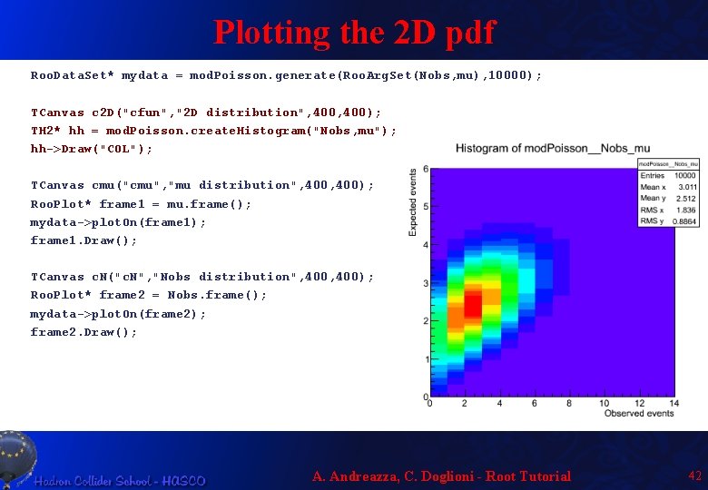
Plotting the 2 D pdf Roo. Data. Set* mydata = mod. Poisson. generate(Roo. Arg. Set(Nobs, mu), 10000); TCanvas c 2 D("cfun", "2 D distribution", 400); TH 2* hh = mod. Poisson. create. Histogram("Nobs, mu"); hh->Draw("COL"); TCanvas cmu("cmu", "mu distribution", 400); Roo. Plot* frame 1 = mu. frame(); mydata->plot. On(frame 1); frame 1. Draw(); TCanvas c. N("c. N", "Nobs distribution", 400); Roo. Plot* frame 2 = Nobs. frame(); mydata->plot. On(frame 2); frame 2. Draw(); A. Andreazza, C. Doglioni - Root Tutorial 42

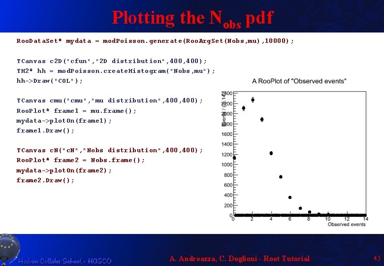
Plotting the Nobs pdf Roo. Data. Set* mydata = mod. Poisson. generate(Roo. Arg. Set(Nobs, mu), 10000); TCanvas c 2 D("cfun", "2 D distribution", 400); TH 2* hh = mod. Poisson. create. Histogram("Nobs, mu"); hh->Draw("COL"); TCanvas cmu("cmu", "mu distribution", 400); Roo. Plot* frame 1 = mu. frame(); mydata->plot. On(frame 1); frame 1. Draw(); TCanvas c. N("c. N", "Nobs distribution", 400); Roo. Plot* frame 2 = Nobs. frame(); mydata->plot. On(frame 2); frame 2. Draw(); A. Andreazza, C. Doglioni - Root Tutorial 43