ROOT Functions Fitting Harinder Singh Bawa California State

ROOT: Functions & Fitting Harinder Singh Bawa California State University Fresno Mar 31, 2016

Review of previous Exercise*: * Good to practice some exercises side by side in order to understand
 Ø Create a gaussian function using TF 1 class of Root, set")
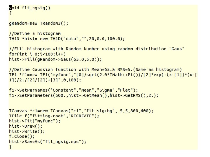
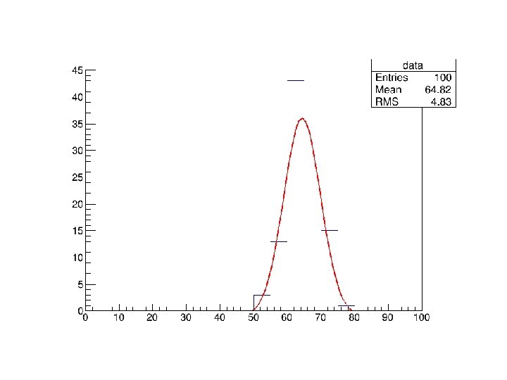
Exercise: 1) Ø Create a gaussian function using TF 1 class of Root, set its parameters(500. , 65. , 5. ), plot it and finally save the plot. Hint: Gaussian function: TF 1 f 1("gauss", "[0] / sqrt(2. 0 * TMath: : Pi()) / [2] * exp(-(x-[1])*(x[1])/2. /[2])", 0, 100) Ø Create a gaussian distributed random numbers using the Random number generator class TRandom 3 and using the provided basic Random distribution "Gaus(mean=65, sigma=5)". Create a 1 dimensional histogram TH 1 D and fill in with the generated random numbers. Finally book a canvas TCanvas and plot the distribution and save it Ø Fit the histogram from (2) with function (1)
 Write a root macro that creates randomly generated data as a signal peak")
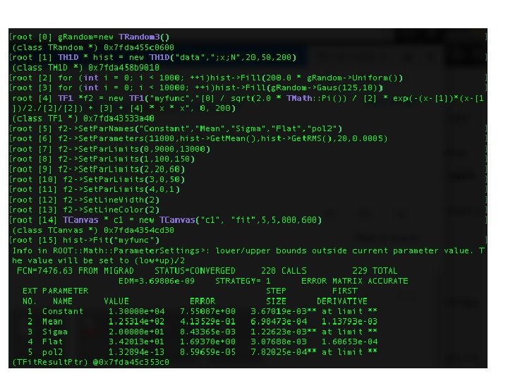
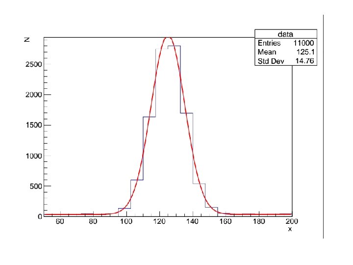
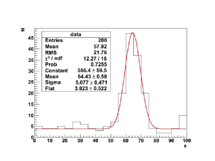
2) Write a root macro that creates randomly generated data as a signal peak (gaussian) with mean= 125. 0 & sigma=10. 0. Perform fit with a gaussian function and inspect the parameters. ØAdd background as uniform ØFit using function gaus+pol 2 ØWrite down the good parameters.
 with a Landau")
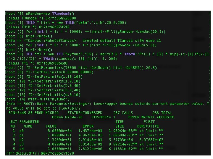
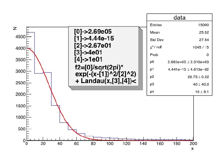
Full Exercise upto now Ø Fill a histogram randomly (n=~10, 000) with a Landau distribution with a most probable value at 20 and a “width” of 5 (use the ROOT website to find out about the Landau function) Ø Fill the same histogram randomly (n=~5, 000) with a Gaussian distribution centered at 5 with a “width” of 3 Ø Write a compiled script with a fit function that describes the total histogram nicely (it might be a good idea to fit both peaks individually first and use the fit parameters for a combined fit) Ø Add titles to x- and y-axis Ø Include a legend of the histogram with number of entries, mean, and RMS values Ø Add text to the canvas with the fitted function parameters Ø Draw everything on a square-size canvas (histogram in blue, fit in red) Ø Save as png, eps, and root file

Simple Straight Line fitting

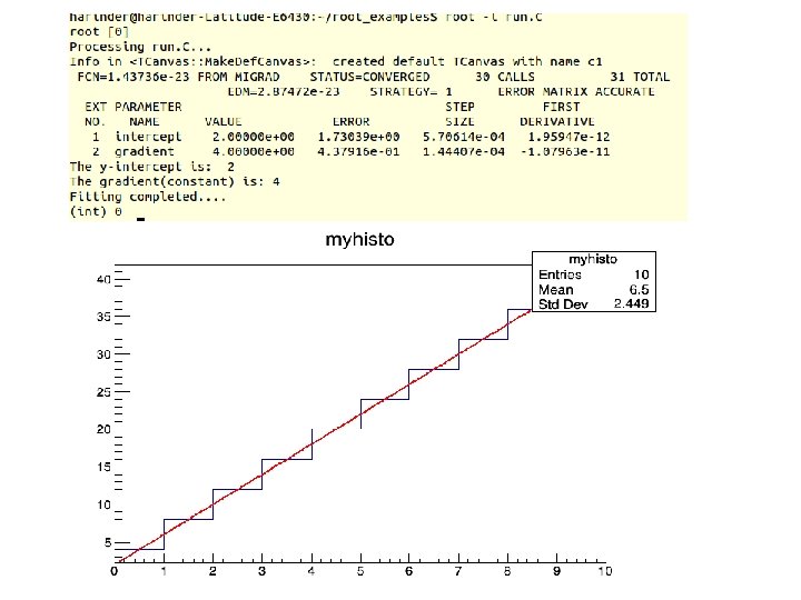
Straight line fit: y=mx + c #include <iostream> #include "TH 1 D. h" #include <TMath. h> #include <TROOT. h> #include "TF 1. h" using namespace std; //Declare a user defined function for fitting Double_t fitf(Double_t *x, Double_t *par) { Double_t value=par[0]+(par[1]*x[0]); //Here par[0]=constant/intercept & par[1] is Gradient return value; } int run(){ //Create a histogram to be fitted TH 1 D* myhisto=new TH 1 D("myhisto", 10, 0, 10); //Fill the histogram for (int i=1; i<=10; i++){ myhisto->Set. Bin. Content(i, i*4); //Randomly }

Contd: //Create a TF 1 object with the function defined above. . //The last three parameters specify the range and number of parameters of the function TF 1 *func=new TF 1("fit", fitf, 0, 10, 2); //Set the initial paramters of the function func->Set. Parameters(0. 04, 0. 1); //Give the parameters meaningful name func->Set. Par. Names("intercept", "gradient"); //Call TH 1: : Fit with the name of TF 1 Object myhisto->Fit("fit"); //Access the Fit results directly cout<<"The y-intercept is: "<<func->Get. Parameter(0)<<endl; cout<<"The gradient(constant) is: "<<func->Get. Parameter(1)<<endl; cout<<"Fitting completed. . "<<endl; return 0; }

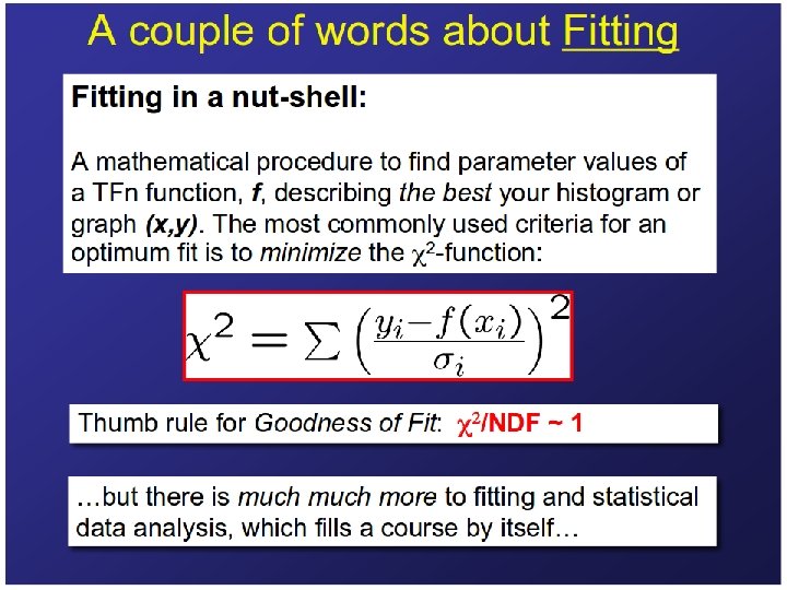
Complex fitting
")
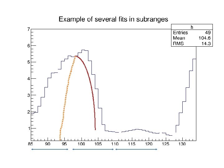
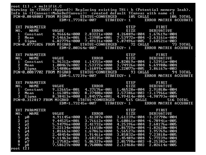
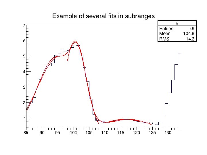
Multi Peak Histogram Fitting #include "TH 1. h" #include "TF 1. h" void multifit() { const Int_t np = 49; Float_t x[np] = {1. 913521, 1. 953769, 2. 347435, 2. 883654, 3. 493567, 4. 047560, 4. 337210, 4. 364347, 4. 563004, 5. 054247, 5. 194183, 5. 380521, 5. 303213, 5. 384578, 5. 563983, 5. 728500, 5. 685752, 5. 080029, 4. 251809, 3. 372246, 2. 207432, 1. 227541, 0. 8597788, 0. 8220503, 0. 8046592, 0. 7684097, 0. 7469761, 0. 8019787, 0. 8362375, 0. 8744895, 0. 9143721, 0. 9462768, 0. 9285364, 0. 8954604, 0. 8410891, 0. 7853871, 0. 7100883, 0. 6938808, 0. 7363682, 0. 7032954, 0. 6029015, 0. 5600163, 0. 7477068, 1. 188785, 1. 938228, 2. 602717, 3. 472962, 4. 465014, 5. 177035}; TH 1 F *h = new TH 1 F("h", "Example of several fits in subranges", np, 85, 134); h->Set. Maximum(7); for (int i=0; i<np; i++) { h->Set. Bin. Content(i+1, x[i]); } h->Draw();
![Fitting (Fitting multiple functions to different ranges of a 1 -D histogram) Double_t par[9];](http://slidetodoc.com/presentation_image/631a14a46306e08d7dce5c8e36b9b5fd/image-19.jpg "Fitting (Fitting multiple functions to different ranges of a 1 -D histogram) Double_t par[9];")
Fitting (Fitting multiple functions to different ranges of a 1 -D histogram) Double_t par[9]; //3 gaussians are fitted in sub-ranges of this histogram TF 1 *g 1 = new TF 1("g 1", "gaus", 85, 95); //sub-Range TF 1 *g 2 = new TF 1("g 2", "gaus", 98, 108); TF 1 *g 3 = new TF 1("g 3", "gaus", 110, 121); //A new function (a sum of 3 gaussians) is fitted on another subrange TF 1 *total = new TF 1("total", "gaus(0)+gaus(3)+gaus(6)", 85, 125); total->Set. Line. Color(2); h->Fit(g 1, "R"); //Fit according to sub-Range only h->Fit(g 2, "R+"); h->Fit(g 3, "R+"); //Note that when fitting simple functions, such as gaussians, the initial values of parameters are automatically computed by ROOT. // In the more complicated case of the sum of 3 gaussians, the initial values of parameters must be given. In this particular case, the initial values are taken from the result of the individual fits g 1 ->Get. Parameters(&par[0]); https: //root. cern. ch/doc/master/class. TF 1. html g 2 ->Get. Parameters(&par[3]); g 3 ->Get. Parameters(&par[6]); total->Set. Parameters(par); h->Fit(total, "R+"); }

Exercise v First create an histogram with a double gaussian peaks and then we fit it. v Create an histogram with 100 bins between 0 and 10. v Fill with 5000 Gaussian number with mean 3 and width 1. 5. v Fill with 5000 Gaussian number with a mean of 8 and width of 1. v Create a function composed of the sum of two Gaussian and fit to the histogram. v Do the fit works ? What do you need to do to make the fit working ?

Hint Before fitting you need to set sensible parameter values. You can do this by fitting first a single Gaussian in the range [0, 5] and then a second Gaussian in the range [5, 10]. If you don't set good initial parameter values, (for example if you set the amplitude of the Gaussians to 1, the means of the Gaussians to 5 and widths to 1), the fit will probably not converge.

BACKUP

Functions

TF 1 with parameters A function can have parameters (e. g. floating parameters for fits. . . )

Let's draw a TF 1 on a TCanvas Like most objects in ROOT, functions can be drawn on a a TCanvas is an object too. . . canvas

Functions and Histograms Ø Define a function: function TF 1 *myfunc=new TF 1(“myfunc”, ”gaus”, 0, 3); Myfunc->Set. Parameters(10. , 1. 5, 0. 5); Myfunc->Draw(); Ø Generate histograms from functions: (Myfunc->Get. Histogram())->Draw(); Ø Generate histograms with random numbers from a function: TH 1 F *hgaus=new TH 1 F(“hgaus”, ”histo from gaus”, 50, 0, 3); hgaus->Fill. Random(“myfunc”, 10000); hgaus->Draw(); Ø Write histogram to a rootfile: TFile *myfile= new Tfile(“hgaus. root”, ”RECREATE”); hgaus->Write(); Myfile->Close();

Fitting Histograms Let us try to fit the histogram created by the previous step: Interactively: § Open rootfile containing histogram: root –l hgaus. root § Draw histogram hgaus->Draw() § Right click on the histogram and select “Fit Panel” § Check to ensure: § “gaus” is selected in the Function->Predefined popmenu § “Chi-square” is selected in the Fit Settings->Method menu § Click on “Fit” at the bottom [Display fit parameters: Select Options->Fit. Parameters]

Fitting contd: Using user defined functions: § Create a file called user_func. C with the following contents: Last 3 parameters specify the number of parameters for the function
 Also can try : g. Style->Set. Opt. Fit(1111)")
g. Style->Set. Opt. Stat(1111111) Also can try : g. Style->Set. Opt. Fit(1111)

Fitting contd: Move the slider to change fit Range

Mean=65, sigma=5.

https: //root. cern. ch/doc/master/class. TRandom. html
- Slides: 36