Root Finding The solution of nonlinear equations and

Root Finding The solution of nonlinear equations and systems Vageli Coutsias, UNM, Fall ‘ 02

The Newton-Raphson iteration for locating zeros

Example: finding the square root Details: initial iterate must be ‘close’ to solution for method to deliver its promise of quadratic convergence (the number of correct bits doubling with every step)

Square root by Newton-Raphson % find square root of A x = (1+2*A)/3; maxiter = 20; for k = 1: maxiter x = (x+ (A/x))/2; end

function x = sqrt 1(A) if A < 0 break; end if A == 0; x = 0; else Two. Power = 1; m = A; while m >= 1, m = m/4; Two. Power = 2*Two. Power ; end while m <. 25, m = m*4; Two. Power = Two. Power/2; end x = (1+2*m)/3; for k = 1: 4 x = (x+ (m/x))/2; end x = x*Two. Power; end

function z = newton(func, z 0, tol, maxiter, varargin) hopt = 2*sqrt(eps); z = z 0; value = feval(func, z, varargin{: }); iter = 1; while abs(value) >=tol deriv = (feval(func, z+hopt, varargin{: }) - val)/hopt; z = z - value/deriv; value = feval(func, z, varargin{: }); iter = iter+1; if iter >= maxiter fprintf('maxiter exceeded, no convergence') break end

function [z, varargout] =. . . newton(func, z 0, tol, maxiter, varargin) hopt = 2*sqrt(eps); z = z 0; iter = 1 value = feval(func, z, varargin{: }); while abs(value) >=tol if iter >= maxiter fprintf('maxiter exceeded, no convergence'); break end deriv = (feval(func, z+hopt, varargin{: }) - val)/hopt; z = z - value/deriv; value = feval(func, z, varargin{: }); iter = iter+1; end if nargout >= 2 ; varargout{1} = val; end if nargout >= 3 ; varargout{2} = iter; end

function zerofinder() clear; close all a=10; b = 3; x = linspace(-20, 100); y = func(x, a, b); zz =zeros(100); plot(x, y, x, zz) [z, val, iter] = newton(@func, 1, . 0001, 40, a, b) function z = func(y, a, b) z=y. ^2+a*y+b; z = -0. 30958376444732 val = 4. 462736 e-006 iter = 4

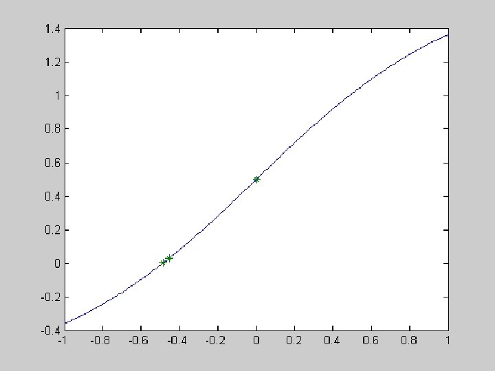
clc; close all; clear all; format long e; fname = 'func'; a = input('Enter a value: '); b = input('Enter b value: '); xc = input('Enter starting value: '); xmax = xc; xmin = xc; fc = feval(fname, xc, a, b); delta =. 0001; fpc = (feval(fname, xc+delta, a, b)-fc)/delta; k=0; disp(sprintf('k x fval fpval ')) while input('Newton step? (0=no, 1=yes)') k=k+1; x(k) = xc; y(k) = fc; xnew = xc – fc / fpc; xc = xnew; fc = feval(fname, xc, a, b); fpc = (feval(fname, xc+delta, a, b)-fc)/delta; disp(sprintf('%2. 0 f %20. 15 f', k, xc, fpc)) if xmax <= x(k); xmax = x(k); end if xmin >= x(k); xmin = x(k); end x 0 = linspace(xmin, xmax, 201); y 0 = feval(fname, x 0, a, b); plot(x 0, y 0, 'r-', x, y, '*')

Enter a value: . 1 Enter b value: . 5 Enter starting value: 0 k x fval Newton step? (0=no, 1=yes)1 1 -0. 45455922915 0. 028917256044793 2 -0. 486015721951951 0. 000349982958035 3 -0. 486406070359515 0. 000000068775315 4 -0. 486406147091071 0. 0000002760 5 -0. 486406147094150 0. 00000000 Newton step? (0=no, 1=yes)0

function f = func(x, a, b) % trap near x = 0 % for interesting behavior, use a =. 1, b =. 0001, x 0 =. 4 f =. 5*x. ^2+ 100*x. ^8 - a*x. ^16 + b;

% script zeroin % uses matlab builtin rootfinder "FZERO" % to find a zero of a function 'fname' close all; clear all; format long %fname = 'func'; % user defined function-can also give as @func %fpname='dfunc'; % user def. derivative-not required by FZERO del =. 0001; % function value limiting tolerance a = input('Enter a value: '); b = input('Enter b value: '); x 0 = linspace(-10, 201); y 0 = feval(@func, x 0, a, b); xc = input('Enter starting value: '); %root = fzero(@func, xc, . 0001, 1, a, b); % grandfathered format OPTIONS=optimset('Max. Iter', 100, 'Tol. Fun', del, 'Tol. X', del^2); root = fzero(@func, xc, OPTIONS, a, b) y = feval(@func, root, a, b) plot(x 0, y 0, root, y, 'r*')

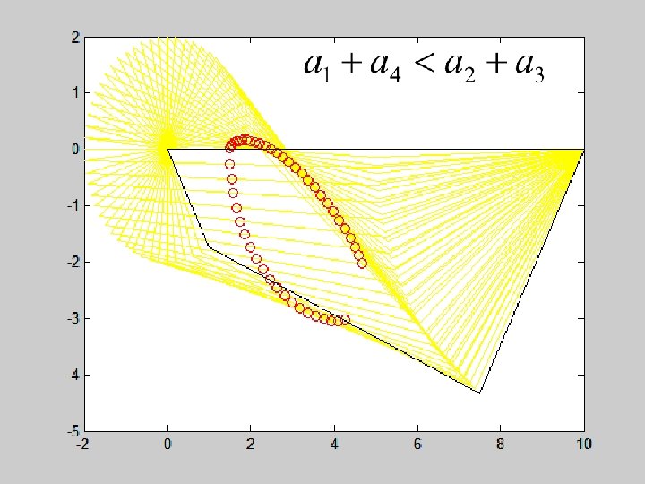
Planar 4 -R linkage

The planar 4 -bar linkage can assume various configurations. For each value of the angle f there are two possible values of y and vice versa. The mid -point of the bar CD executes a complex motion.

function linkage() close all; a 1=10; a 2=5; a 3=7; a 4=2; psi 0=30; A=[0, 0]; B=[a 1, 0]; axis equal for i = 1: 60 phi(i)=i*pi/30; psi(i) = fzero(@bar 4, psi 0, [], phi(i), a 1, a 2, a 3, a 4); C=[a 1+a 2*cos(psi(i)), a 2*sin(psi(i))]; D= [a 4*cos(phi(i)), a 4*sin(phi(i))]; XX=[A, B, C, D, A]; plot(XX(: , 1), XX(: , 2), 'k-') hold on x = (a 1+a 2*cos(psi)+a 4*cos(phi))/2; y = (a 2*sin(psi)+a 4*sin(phi))/2; plot(x, y, 'ro'); pause(. 1) plot(XX(: , 1), XX(: , 2), 'y-') end plot(XX(: , 1), XX(: , 2), 'k-')

D traces full circle about A

Application: solution of a BVP (Boundary Value Problem) Solution

Problem Solve previous equation for the smallest suitable nonzero value of k (eigenvalue) using (a) The Newton method (script ‘NEWT. M’) (b) The built-in Newton method (script ‘ZEROIN. M’) (c) The secant method (script ‘SEC. M’)

FIXED POINT ITERATIONS Unique fixed point in interval [a, b]

fixed-point iteration: the idea

Error estimate use difference between successive iterates to estimate error

Newton iteration as fixed-point iteration: quadratic convergence

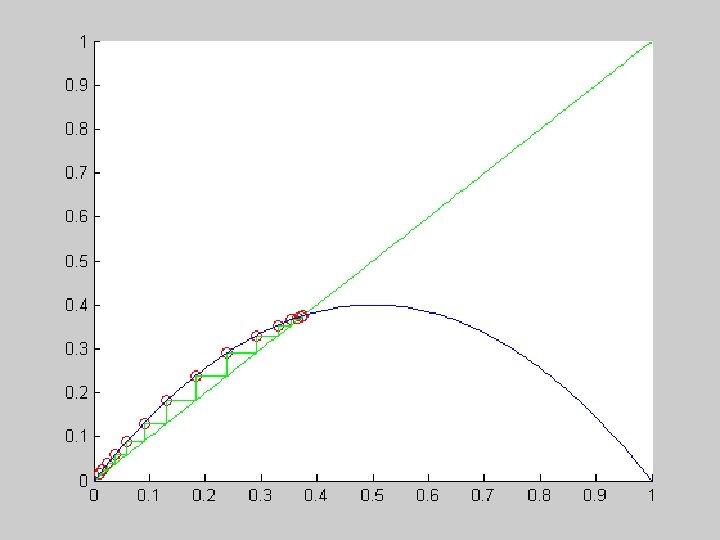
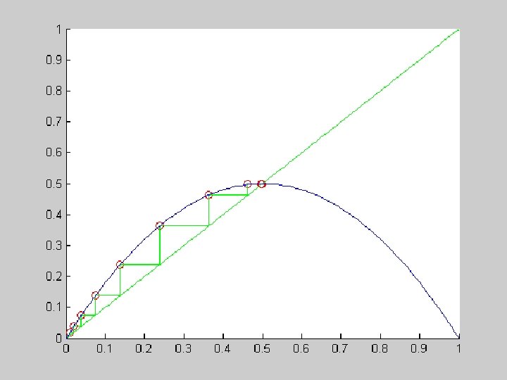
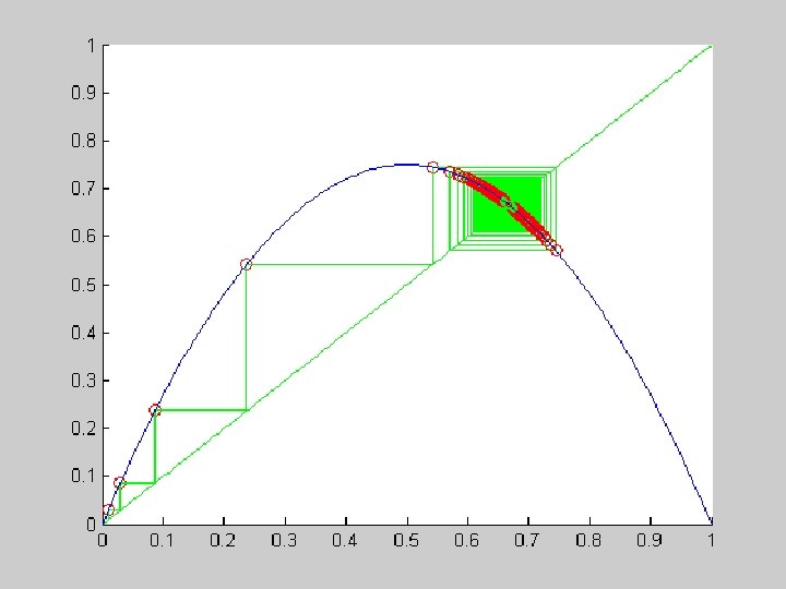
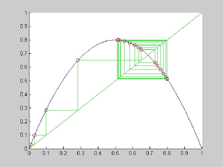
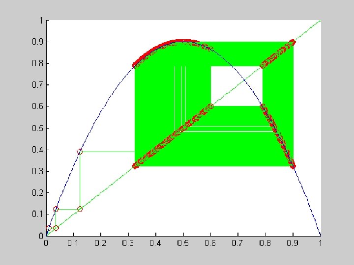
Example: the logistic map What happens if uniqueness is violated?

function fixed_point() close all a =. 9; tol = 10^(-16); imax = 1000; i = 1; deltax = 1; x(1) =. 01; while deltax >= tol & i <= imax x(i+1) = f 1(x(i), a); deltax = abs(x(i+1)-x(i)); i = i+1; end n = length(x) xx = linspace(0, 1, 100); yy = f 1(xx, a); plot(xx, 'g', xx, yy, 'b', x(1: n-1), x(2, n), 'ro') function y = f 1(x, a) y = 4*a*x. *(1 -x);

a=. 2: unique fixed point at x=0

a=. 4

a=. 5

a=. 75: slow convergence

a=. 8: fixed point of order 2

a=. 875: fixed point of order 4

a=. 89: order 8

a=. 9: no fixed points (chaos)

a=. 95

FMINBND Scalar bounded nonlinear function minimization. X = FMINBND(FUN, x 1, x 2) starts at X 0 and finds a local minimizer X of the function FUN in the interval x 1 < X < x 2. FUN accepts scalar input X and returns a scalar function value F evaluated at X.

SPLINE Cubic spline data interpolation. YY = SPLINE(X, Y, XX) uses cubic spline interpolation to find YY, the values of the underlying function Y at the points in the vector XX. The vector X specifies the points at which the data Y is given. If Y is a matrix, then the data is taken to be vector-valued and interpolation is performed for each column of Y and YY will be length(XX)-by-size(Y, 2). PP = SPLINE(X, Y) returns the piecewise polynomial form of the cubic spline interpolant for later use with PPVAL and the spline utility UNMKPP. Ordinarily, the not-a-knot end conditions are used. However, if Y contains two more values than X has entries, then the first and last value in Y are used as the endslopes for the cubic spline. Namely: f(X) = Y(: , 2: end-1), df(min(X)) = Y(: , 1), df(max(X)) = Y(: , end) Example: This generates a sine curve, then samples the spline over a finer mesh: x = 0: 10; y = sin(x); xx = 0: . 25: 10; yy = spline(x, y, xx); plot(x, y, 'o', xx, yy)

PPVAL Evaluate piecewise polynomial. V = PPVAL(PP, XX) returns the value at the points XX of the piecewise polynomial contained in PP, as constructed by SPLINE or the spline utility MKPP. V = PPVAL(XX, PP) is also acceptable, and of use in conjunction with FMINBND, FZERO, QUAD, and other functions. Example: Compare the results of integrating the function cos and this spline: a = 0; b = 10; int 1 = quad(@cos, a, b, []); x = a : b; y = cos(x); pp = spline(x, y); int 2 = quad(@ppval, a, b, [], pp); int 1 provides the integral of the cosine function over the interval [a, b] while int 2 provides the integral over the same interval of the piecewise polynomial pp which approximates the cosine function by interpolating the computed x, y values.

The Secant iteration for locating zeros

% script SEC. M: uses secant method to find zero of FUNC. M close all; clear all; clc; format long e fname = 'func'; a = input('Enter a: '); b = input('Enter b: '); xc = input('Enter starting value: '); fc = feval(fname, xc, a, b); del =. 0001; k=0; disp(sprintf('k x fval fpval ')) fpc = (feval(fname, xc+delta, a, b)-fc)/delta; while input('secant step? (0=no, 1=yes)') k=k+1; x(k) = xc; y(k) = fc; f_ = fc; xnew = xc - fc/fpc; x_ = xc; xc = xnew; fc = feval(fname, xc, a, b); fpc= (fc - f_)/(xc-x_); disp(sprintf('%2. 0 f %20. 15 f', k, xc, fpc)) end if x(1) <= x(k); xa = floor(x(1)-. 5); xb = ceil(x(k)+. 5); else; xb = floor(x(1)-. 5); xa = ceil(x(k)+. 5); end x 0=linspace(xa, xb, 201); y 0=feval(fname, x 0, a, b); plot(x 0, y 0, x, y, 'r*')