ROMS Framework and Algorithms Hernan G Arango Institute

ROMS Framework and Algorithms Hernan G. Arango Institute of Marine and Coastal Sciences Rutgers University, New Brunswick, NJ, USA ROMS/TOMS Asia-Pacific Workshop Sydney Institute of Marine Science, Sydney Australia April 1, 2009

Outline • Vertical Coordinate Transformation Revisited • Advection Operator • Matlab Processing Scripts Repository • Serial and Parallel I/O • Data Assimilation Algorithms

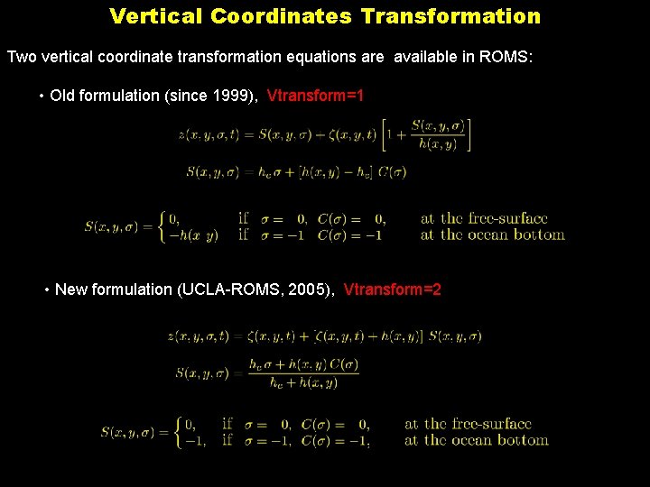
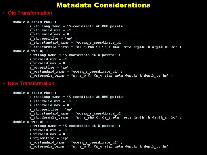
Vertical Coordinates Transformation Two vertical coordinate transformation equations are available in ROMS: • Old formulation (since 1999), Vtransform=1 • New formulation (UCLA-ROMS, 2005), Vtransform=2

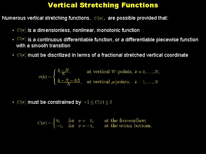
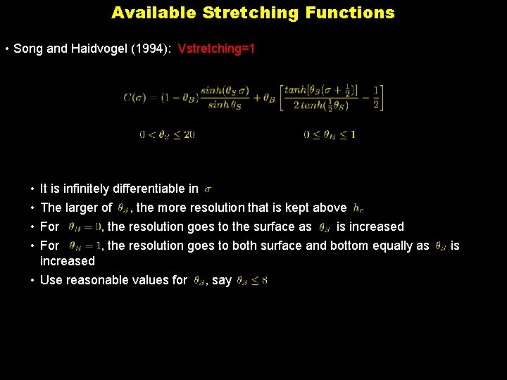
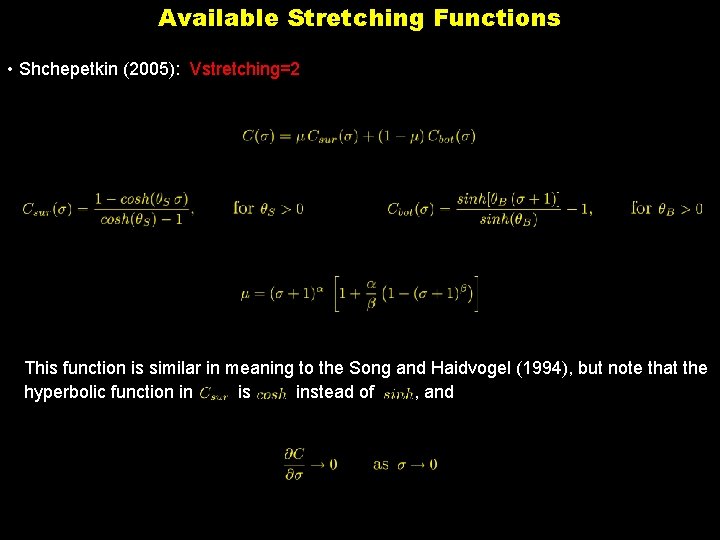
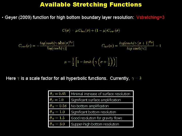
Vertical Stretching Functions Numerous vertical stretching functions, • , are possible provided that: is a dimensionless, nonlinear, monotonic function • is a continuous differentiable function, or a differentiable piecewise function with a smooth transition • must be discritized in terms of a fractional stretched vertical coordinate • must be constrained by

Available Stretching Functions • Song and Haidvogel (1994): Vstretching=1 • • It is infinitely differentiable in The larger of , the more resolution that is kept above For , the resolution goes to the surface as is increased For , the resolution goes to both surface and bottom equally as increased • Use reasonable values for , say is

Available Stretching Functions • Shchepetkin (2005): Vstretching=2 This function is similar in meaning to the Song and Haidvogel (1994), but note that the hyperbolic function in is instead of , and

Available Stretching Functions • Geyer (2009) function for high bottom boundary layer resolution: Vstretching=3 Here is a scale factor for all hyperbolic functions. Currently, Minimal increase of surface resolution Significant surface amplification No bottom amplification Significant bottom resolution Good resolution for gravity flows Supper-high bottom resolution

Metadata Considerations • Old Transformation double s_rho(s_rho) ; s_rho: long_name = "S-coordinate at RHO-points" ; s_rho: valid_min = -1. ; s_rho: valid_max = 0. ; s_rho: positive = "up" ; s_rho: standard_name = "ocean_s_coordinate_g 1" ; s_rho: formula_terms = "s: s_rho C: Cs_r eta: zeta depth: h depth_c: hc" ; double s_w(s_w) ; s_w: long_name = "S-coordinate at W-points" ; s_w: valid_min = -1. ; s_w: valid_max = 0. ; s_w: positive = "up" ; s_w: standard_name = "ocean_s_coordinate_g 1" ; s_w: formula_terms = "s: s_w C: Cs_w eta: zeta depth: h depth_c: hc" ; • New Transformation double s_rho(s_rho) ; s_rho: long_name = "S-coordinate at RHO-points" ; s_rho: valid_min = -1. ; s_rho: valid_max = 0. ; s_rho: positive = "up" ; s_rho: standard_name = "ocean_s_coordinate_g 2" ; s_rho: formula_terms = "s: s_rho C: Cs_r eta: zeta depth: h depth_c: hc" ; double s_w(s_w) ; s_w: long_name = "S-coordinate at W-points" ; s_w: valid_min = -1. ; s_w: valid_max = 0. ; s_w: positive = "up" ; s_w: standard_name = "ocean_s_coordinate_g 2" ; s_w: formula_terms = "s: s_w C: Cs_w eta: zeta depth: h depth_c: hc" ;

Standard Input File: ocean. in

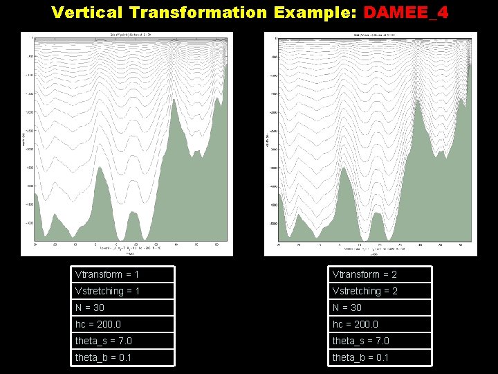
Vertical Transformation Example: DAMEE_4 Vtransform = 1 Vtransform = 2 Vstretching = 1 Vstretching = 2 N = 30 hc = 200. 0 theta_s = 7. 0 theta_b = 0. 1

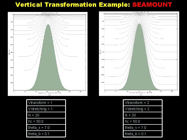
Vertical Transformation Example: SEAMOUNT Vtransform = 1 Vtransform = 2 Vstretching = 1 Vstretching = 2 N = 20 hc = 50. 0 theta_s = 7. 0 theta_b = 0. 1

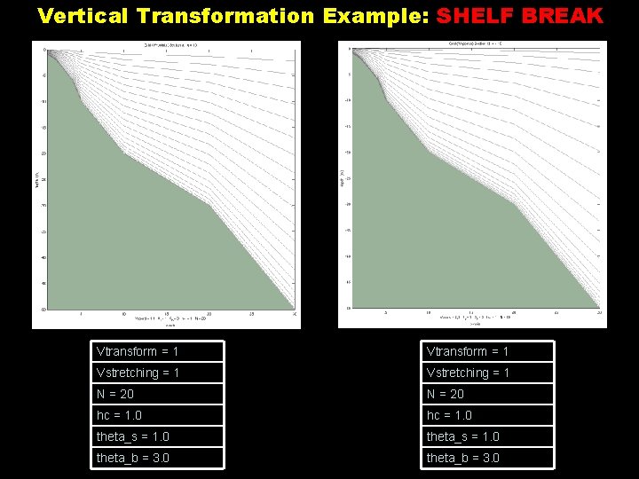
Vertical Transformation Example: SHELF BREAK Vtransform = 1 Vstretching = 1 N = 20 hc = 1. 0 theta_s = 1. 0 theta_b = 3. 0

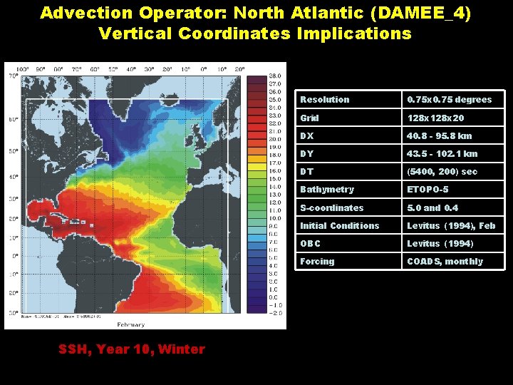
Advection Operator: North Atlantic (DAMEE_4) Vertical Coordinates Implications SSH, Year 10, Winter Resolution 0. 75 x 0. 75 degrees Grid 128 x 20 DX 40. 8 - 95. 8 km DY 43. 5 - 102. 1 km DT (5400, 200) sec Bathymetry ETOPO-5 S-coordinates 5. 0 and 0. 4 Initial Conditions Levitus (1994), Feb OBC Levitus (1994) Forcing COADS, monthly

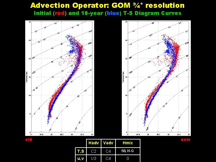
Advection Operator: GOM ¾° resolution Initial (red) and 10 -year (blue) T-S Diagram Curves old Hadv Vadv Hmix T, S C 2 C 4 50, H-G u, v U 3 C 4 0 new

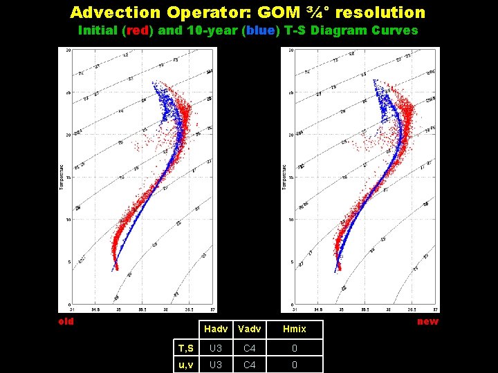
Advection Operator: GOM ¾° resolution Initial (red) and 10 -year (blue) T-S Diagram Curves old Hadv Vadv Hmix T, S U 3 C 4 0 u, v U 3 C 4 0 new

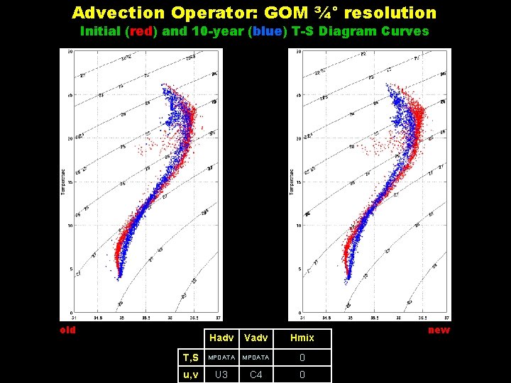
Advection Operator: GOM ¾° resolution Initial (red) and 10 -year (blue) T-S Diagram Curves old Hadv Vadv Hmix T, S MPDATA 0 u, v U 3 C 4 0 new

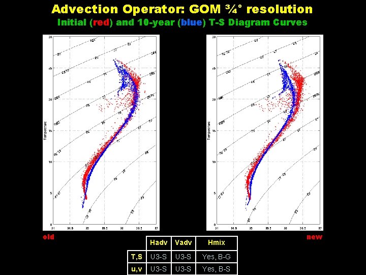
Advection Operator: GOM ¾° resolution Initial (red) and 10 -year (blue) T-S Diagram Curves old Hadv Vadv Hmix T, S U 3 -S Yes, B-G u, v U 3 -S Yes, B-S new

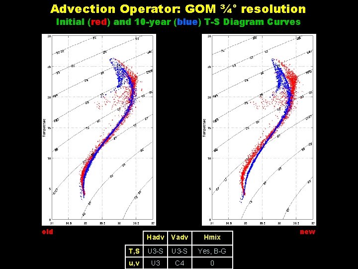
Advection Operator: GOM ¾° resolution Initial (red) and 10 -year (blue) T-S Diagram Curves old Hadv Vadv Hmix T, S U 3 -S Yes, B-G u, v U 3 C 4 0 new

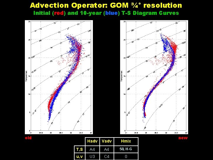
Advection Operator: GOM ¾° resolution Initial (red) and 10 -year (blue) T-S Diagram Curves old Hadv Vadv Hmix T, S A 4 50, H-G u, v U 3 C 4 0 new

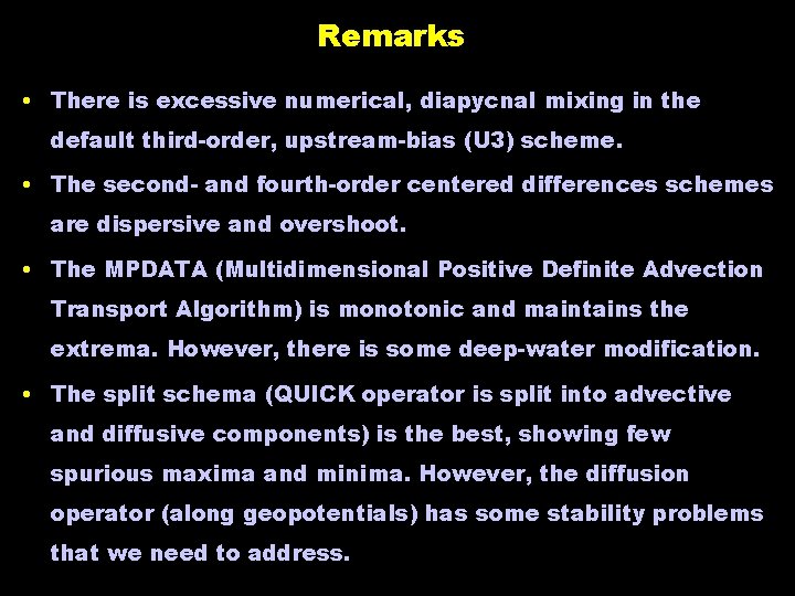
Remarks • There is excessive numerical, diapycnal mixing in the default third-order, upstream-bias (U 3) scheme. • The second- and fourth-order centered differences schemes are dispersive and overshoot. • The MPDATA (Multidimensional Positive Definite Advection Transport Algorithm) is monotonic and maintains the extrema. However, there is some deep-water modification. • The split schema (QUICK operator is split into advective and diffusive components) is the best, showing few spurious maxima and minima. However, the diffusion operator (along geopotentials) has some stability problems that we need to address.

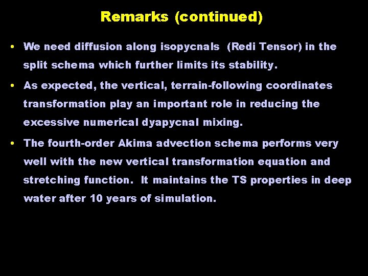
Remarks (continued) • We need diffusion along isopycnals (Redi Tensor) in the split schema which further limits stability. • As expected, the vertical, terrain-following coordinates transformation play an important role in reducing the excessive numerical dyapycnal mixing. • The fourth-order Akima advection schema performs very well with the new vertical transformation equation and stretching function. It maintains the TS properties in deep water after 10 years of simulation.

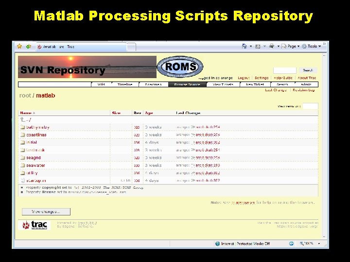
Matlab Processing Scripts Repository

Set_depth. m

stretching. m

scoord. m

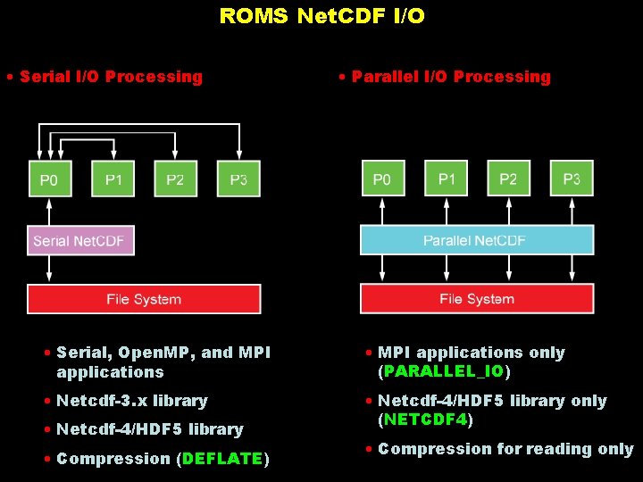
ROMS Net. CDF I/O • Serial I/O Processing • Parallel I/O Processing • Serial, Open. MP, and MPI applications • MPI applications only (PARALLEL_IO) • Netcdf-3. x library • Netcdf-4/HDF 5 library only (NETCDF 4) • Netcdf-4/HDF 5 library • Compression (DEFLATE) • Compression for reading only

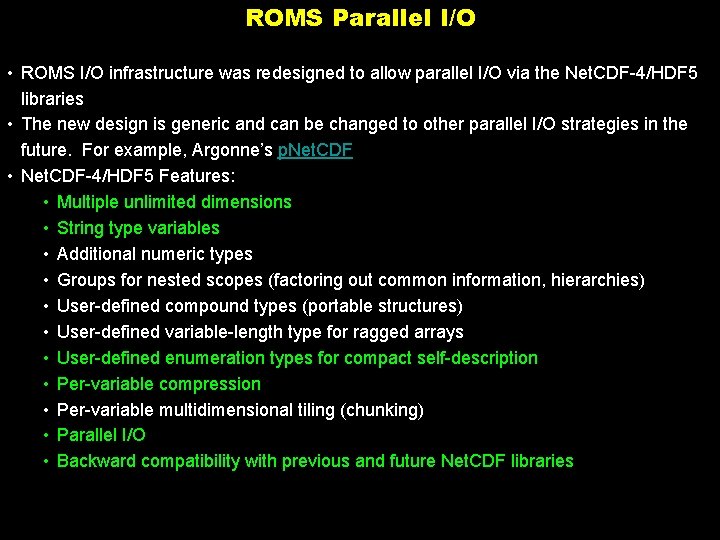
ROMS Parallel I/O • ROMS I/O infrastructure was redesigned to allow parallel I/O via the Net. CDF-4/HDF 5 libraries • The new design is generic and can be changed to other parallel I/O strategies in the future. For example, Argonne’s p. Net. CDF • Net. CDF-4/HDF 5 Features: • Multiple unlimited dimensions • String type variables • Additional numeric types • Groups for nested scopes (factoring out common information, hierarchies) • User-defined compound types (portable structures) • User-defined variable-length type for ragged arrays • User-defined enumeration types for compact self-description • Per-variable compression • Per-variable multidimensional tiling (chunking) • Parallel I/O • Backward compatibility with previous and future Net. CDF libraries

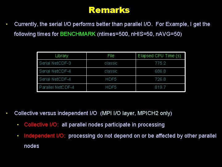
Remarks • Currently, the serial I/O performs better than parallel I/O. For Example, I get the following times for BENCHMARK (ntimes=500, n. HIS=50, n. AVG=50) Library • File Elapsed CPU Time (s) Serial Net. CDF-3 classic 775. 2 Serial Net. CDF-4 classic 686. 8 Serial Net. CDF-4 HDF 5 726. 8 Parallel Net. CDF-4 HDF 5 819. 7 Collective versus independent I/O (MPI I/O layer, MPICH 2 only) • Collective I/O: all parallel nodes participate in processing • Independent I/O: processing do not depend on or be affected by other parallel nodes

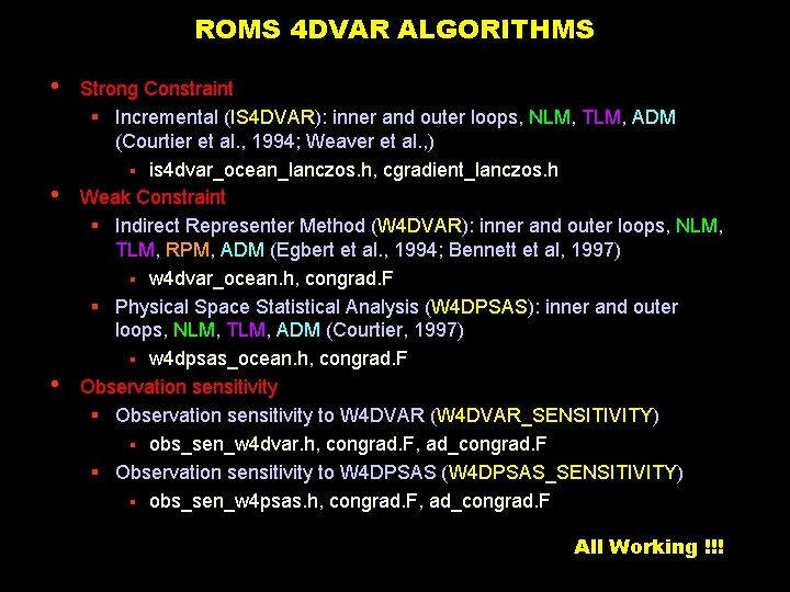
ROMS 4 DVAR ALGORITHMS • • • Strong Constraint § Incremental (IS 4 DVAR): inner and outer loops, NLM, TLM, ADM (Courtier et al. , 1994; Weaver et al. , ) § is 4 dvar_ocean_lanczos. h, cgradient_lanczos. h Weak Constraint § Indirect Representer Method (W 4 DVAR): inner and outer loops, NLM, TLM, RPM, ADM (Egbert et al. , 1994; Bennett et al, 1997) § w 4 dvar_ocean. h, congrad. F § Physical Space Statistical Analysis (W 4 DPSAS): inner and outer loops, NLM, TLM, ADM (Courtier, 1997) § w 4 dpsas_ocean. h, congrad. F Observation sensitivity § Observation sensitivity to W 4 DVAR (W 4 DVAR_SENSITIVITY) § obs_sen_w 4 dvar. h, congrad. F, ad_congrad. F § Observation sensitivity to W 4 DPSAS (W 4 DPSAS_SENSITIVITY) § obs_sen_w 4 psas. h, congrad. F, ad_congrad. F All Working !!!

4 DVAR Data Assimilation Algorithms • Spectral and Ritz pre-conditioning based on the Lanczos algorithm: – https: //www. myroms. org/wiki/index. php/Variational_Data_Assimilation • 4 DVAR state vector: – Initial conditions adjustment – Boundary conditions adjustment – Surface forcing adjustment: wind stress, surface net heat flux, surface freshwater flux, … – Interior model adjustment, weak constraint • Balance Operator

s 4 dvar. in

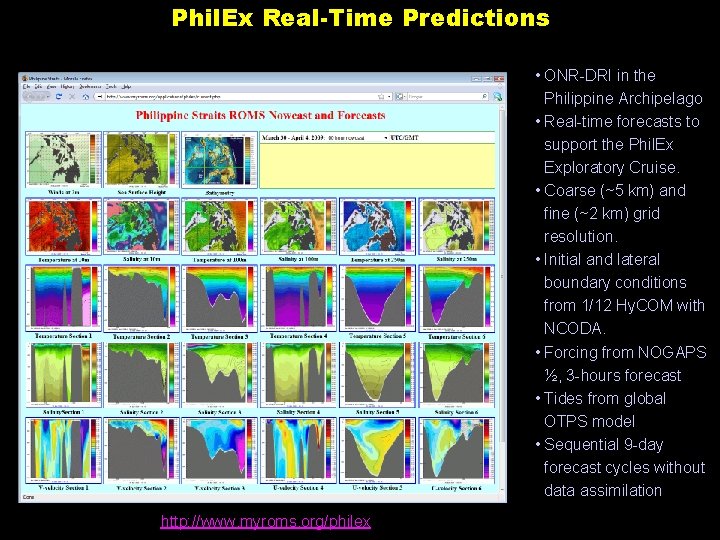
Phil. Ex Real-Time Predictions • ONR-DRI in the Philippine Archipelago • Real-time forecasts to support the Phil. Ex Exploratory Cruise. • Coarse (~5 km) and fine (~2 km) grid resolution. • Initial and lateral boundary conditions from 1/12 Hy. COM with NCODA. • Forcing from NOGAPS ½, 3 -hours forecast • Tides from global OTPS model • Sequential 9 -day forecast cycles without data assimilation http: //www. myroms. org/philex

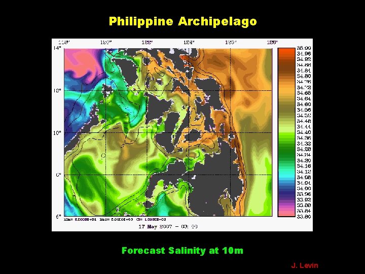
Philippine Archipelago Forecast Salinity at 10 m J. Levin

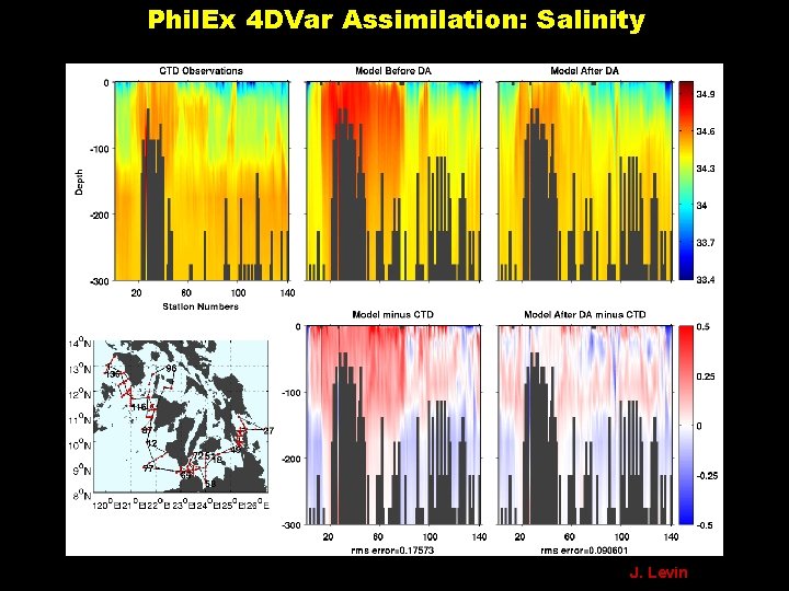
Phil. Ex 4 DVar Assimilation: Salinity J. Levin

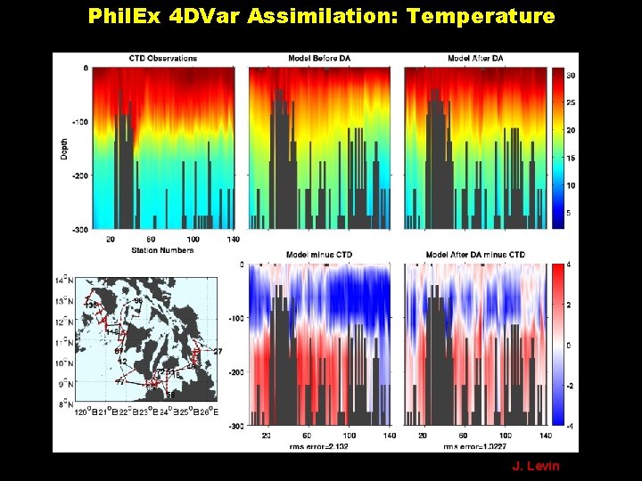
Phil. Ex 4 DVar Assimilation: Temperature J. Levin

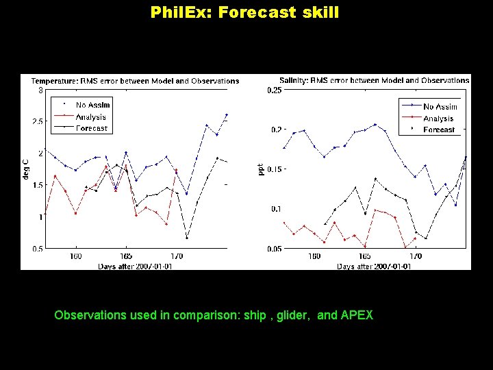
Phil. Ex: Forecast skill Observations used in comparison: ship , glider, and APEX

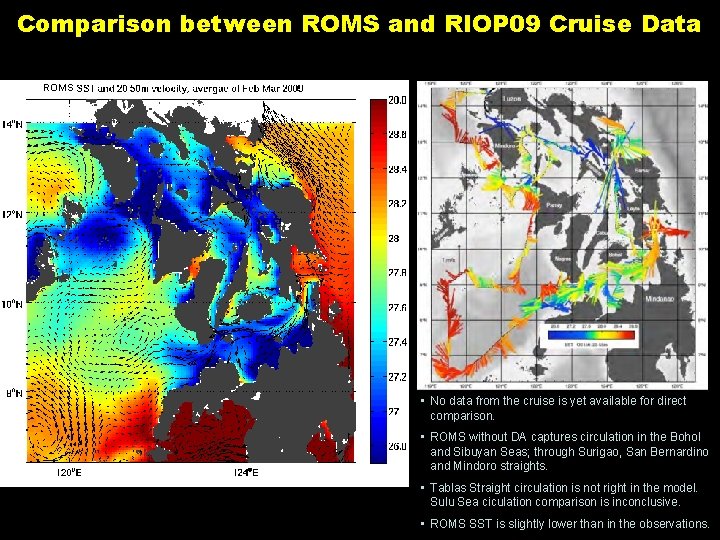
Comparison between ROMS and RIOP 09 Cruise Data SST and 22 -55 m velocity (from A. Gordon) ROMS • No data from the cruise is yet available for direct comparison. • ROMS without DA captures circulation in the Bohol and Sibuyan Seas; through Surigao, San Bernardino and Mindoro straights. • Tablas Straight circulation is not right in the model. Sulu Sea ciculation comparison is inconclusive. • ROMS SST is slightly lower than in the observations.

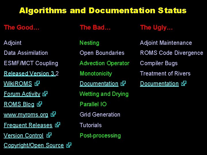
Algorithms and Documentation Status The Good… The Bad… The Ugly… Adjoint Nesting Adjoint Maintenance Data Assimilation Open Boundaries ROMS Code Divergence ESMF/MCT Coupling Advection Operator Compiler Bugs Released Version 3. 2 Monotonicity Treatment of Rivers Wiki. ROMS Documentation Forum Activity Wetting and Drying ROMS Blog Parallel IO www. myroms. org Grid Generation Frequent Releases Tutorials Version Control Post-processing Copyright/Open Source