ROMS Framework and Algorithms Hernan G Arango IMCS

ROMS Framework and Algorithms Hernan G. Arango IMCS, Rutgers Bruce D. Cornuelle SIO, UCSD John L. Wilkin IMCS, Rutgers Emanuele Di Lorenzo Georgia Tech Javier Zavala-Garay IMCS, Rutgers Arthur J. Miller SIO, UCSD Andrew M. Moore UCSC ROMS/TOMS European Workshop Alcala de Henares, Spain, November 7, 2006

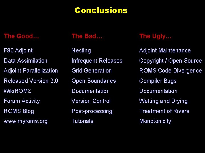
Conclusions The Good… The Bad… The Ugly… F 90 Adjoint Nesting Adjoint Maintenance Data Assimilation Infrequent Releases Copyright / Open Source Adjoint Parallelization Grid Generation ROMS Code Divergence Released Version 3. 0 Open Boundaries Compiler Bugs Wiki. ROMS Documentation Forum Activity Version Control Wetting and Drying ROMS Blog Post-processing Treatment of Rivers www. myroms. org Tutorials Monotonicity

ROMS Framework

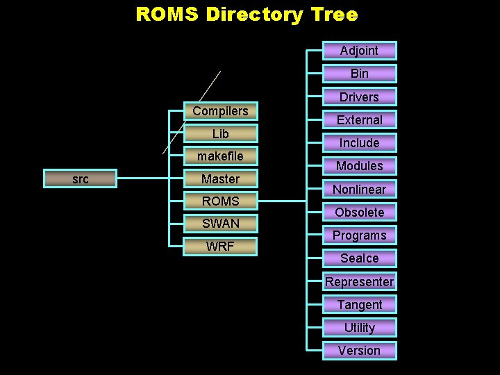
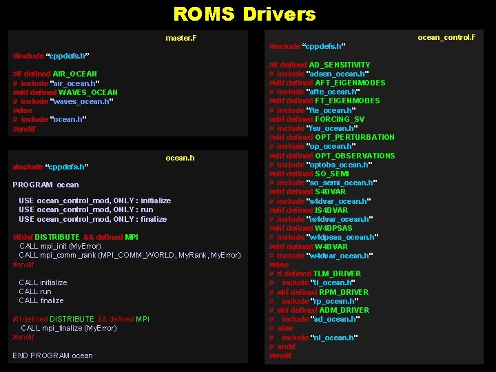
ROMS Directory Tree Adjoint Bin Drivers Compilers Lib makefile src Master ROMS SWAN WRF External Include Modules Nonlinear Obsolete Programs Sea. Ice Representer Tangent Utility Version

ROMS Drivers ocean_control. F master. F #include “cppdefs. h” #if defined AIR_OCEAN # include "air_ocean. h" #elif defined WAVES_OCEAN # include "waves_ocean. h" #else # include "ocean. h" #endif ocean. h #include “cppdefs. h” PROGRAM ocean USE ocean_control_mod, ONLY : initialize USE ocean_control_mod, ONLY : run USE ocean_control_mod, ONLY : finalize #ifdef DISTRIBUTE && defined MPI CALL mpi_init (My. Error) CALL mpi_comm_rank (MPI_COMM_WORLD, My. Rank, My. Error) #endif CALL initialize CALL run CALL finalize #if defined DISTRIBUTE && defined MPI CALL mpi_finalize (My. Error) #endif END PROGRAM ocean #if defined AD_SENSITIVITY # include "adsen_ocean. h" #elif defined AFT_EIGENMODES # include "afte_ocean. h" #elif defined FT_EIGENMODES # include "fte_ocean. h" #elif defined FORCING_SV # include "fsv_ocean. h" #elif defined OPT_PERTURBATION # include "op_ocean. h" #elif defined OPT_OBSERVATIONS # include "optobs_ocean. h" #elif defined SO_SEMI # include "so_semi_ocean. h" #elif defined S 4 DVAR # include "s 4 dvar_ocean. h" #elif defined IS 4 DVAR # include "is 4 dvar_ocean. h" #elif defined W 4 DPSAS # include "w 4 dpsas_ocean. h" #elif defined W 4 DVAR # include "w 4 dvar_ocean. h" #else # if defined TLM_DRIVER # include "tl_ocean. h" # elif defined RPM_DRIVER # include "rp_ocean. h" # elif defined ADM_DRIVER # include "ad_ocean. h" # else # include "nl_ocean. h" # endif #endif

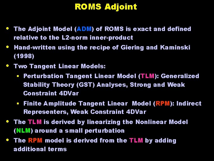
ROMS Adjoint • The Adjoint Model (ADM) of ROMS is exact and defined relative to the L 2 -norm inner-product • Hand-written using the recipe of Giering and Kaminski (1998) • Two Tangent Linear Models: § Perturbation Tangent Linear Model (TLM): Generalized Stability Theory (GST) Analyses, Strong and Weak Constraint 4 DVar § Finite Amplitude Tangent Linear Model (RPM): Indirect Representers, Weak Constraint 4 DVar • The TLM is derived by linearizing the Nonlinear Model (NLM) around a small perturbation • The RPM model is derived from the TLM by adding additional terms

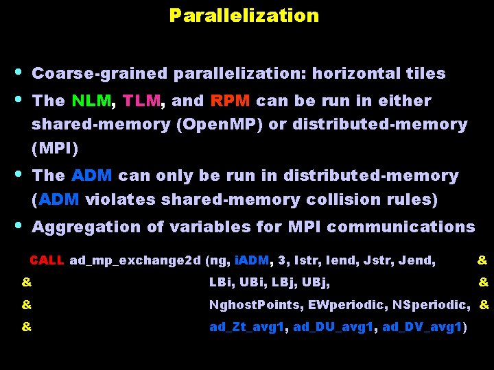
Parallelization • Coarse-grained parallelization: horizontal tiles • The NLM, TLM, and RPM can be run in either shared-memory (Open. MP) or distributed-memory (MPI) • The ADM can only be run in distributed-memory (ADM violates shared-memory collision rules) • Aggregation of variables for MPI communications CALL ad_mp_exchange 2 d (ng, i. ADM, 3, Istr, Iend, Jstr, Jend, & & LBi, UBi, LBj, UBj, & & Nghost. Points, EWperiodic, NSperiodic, & & ad_Zt_avg 1, ad_DU_avg 1, ad_DV_avg 1)

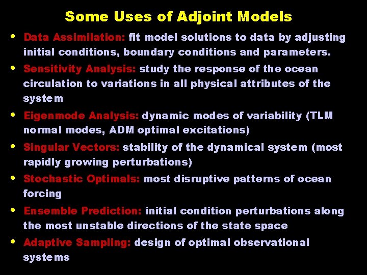
Some Uses of Adjoint Models • Data Assimilation: fit model solutions to data by adjusting initial conditions, boundary conditions and parameters. • Sensitivity Analysis: study the response of the ocean circulation to variations in all physical attributes of the system • Eigenmode Analysis: dynamic modes of variability (TLM normal modes, ADM optimal excitations) • Singular Vectors: stability of the dynamical system (most rapidly growing perturbations) • Stochastic Optimals: most disruptive patterns of ocean forcing • Ensemble Prediction: initial condition perturbations along the most unstable directions of the state space • Adaptive Sampling: design of optimal observational systems

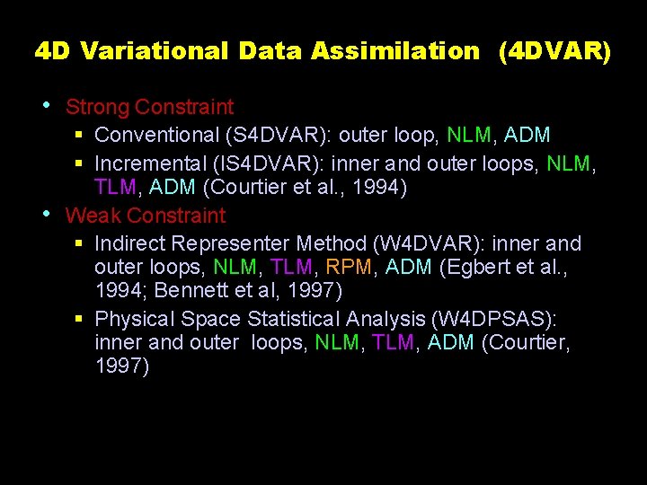
4 D Variational Data Assimilation (4 DVAR) • Strong Constraint § Conventional (S 4 DVAR): outer loop, NLM, ADM § Incremental (IS 4 DVAR): inner and outer loops, NLM, TLM, ADM (Courtier et al. , 1994) • Weak Constraint § Indirect Representer Method (W 4 DVAR): inner and outer loops, NLM, TLM, RPM, ADM (Egbert et al. , 1994; Bennett et al, 1997) § Physical Space Statistical Analysis (W 4 DPSAS): inner and outer loops, NLM, TLM, ADM (Courtier, 1997)

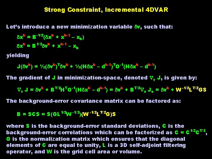
Strong Constraint, Incremental 4 DVAR Let’s introduce a new minimization variable v, such that: xk = B-1/2( xk + xk-1 – xb) xk = B 1/2 vk + xk-1 – xb yielding J( vk) = ½( vk)T vk + ½(H xk – dk-1)TO-1(H xk – dk-1) The gradient of J in minimization-space, denoted v J, is given by: v J = vk + BT/2 HTO-1(H xk – dk-1) = vk + BT/2 x Jo = vk + W -1/2 LT/2 GS The background-error covariance matrix can be factored as: B = SCS = S(GL 1/2 W -1/2)(W -1/2 LT/2 G)S where S is the background-error standard deviations, C is the background-error correlations which can be factorized as C = C 1/2 CT/2, G is the normalization matrix which ensures that the diagonal elements of C are equal to unity, L is a 3 D self-adjoint filtering operator, and W is the grid cell area or volume.

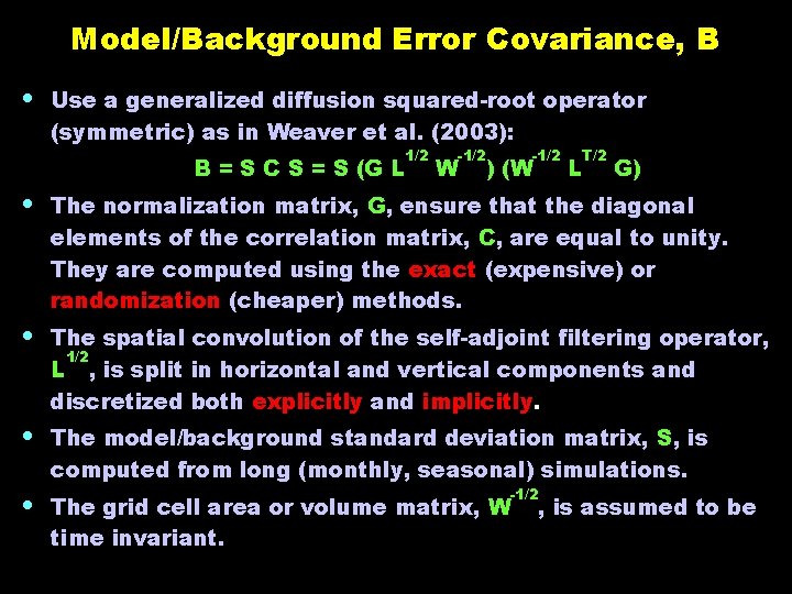
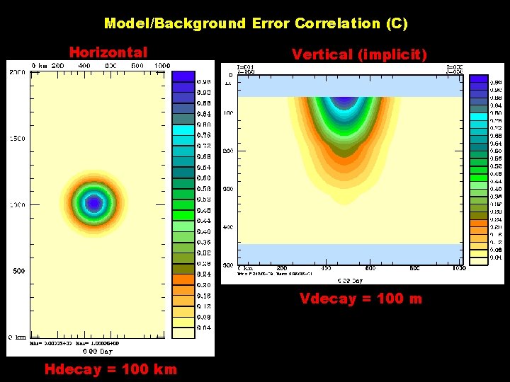
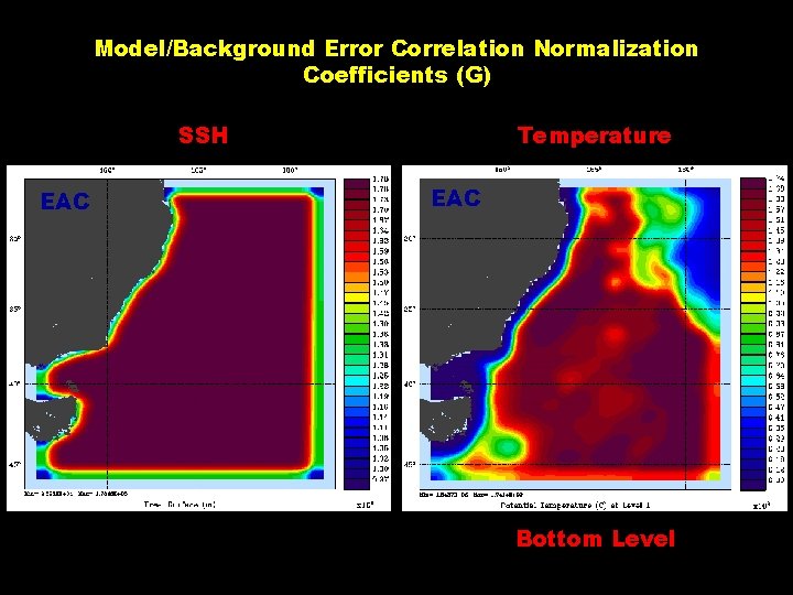
Model/Background Error Covariance, B • Use a generalized diffusion squared-root operator (symmetric) as in Weaver et al. (2003): B = S C S = S (G L 1/2 W -1/2 ) (W -1/2 L T/2 G) • The normalization matrix, G, ensure that the diagonal elements of the correlation matrix, C, are equal to unity. They are computed using the exact (expensive) or randomization (cheaper) methods. • The spatial convolution of the self-adjoint filtering operator, 1/2 L , is split in horizontal and vertical components and discretized both explicitly and implicitly. • The model/background standard deviation matrix, S, is computed from long (monthly, seasonal) simulations. -1/2 • The grid cell area or volume matrix, W time invariant. , is assumed to be

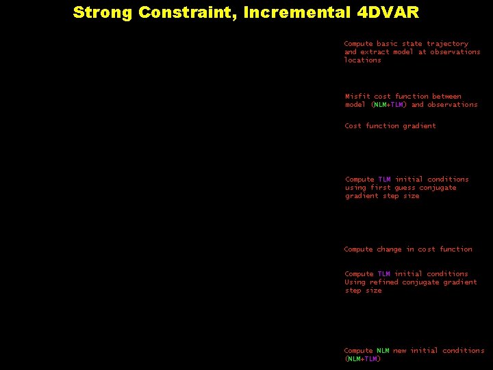
Strong Constraint, Incremental 4 DVAR Compute basic state trajectory and extract model at observations locations Misfit cost function between model (NLM+TLM) and observations Cost function gradient Compute TLM initial conditions using first guess conjugate gradient step size Compute change in cost function Compute TLM initial conditions Using refined conjugate gradient step size Compute NLM new initial conditions (NLM+TLM)

Model/Background Error Correlation (C) Horizontal Vertical (implicit) Vdecay = 100 m Hdecay = 100 km

Model/Background Error Correlation Normalization Coefficients (G) SSH EAC Temperature EAC Bottom Level

Generalized Stability Theory (GST) • Dynamics/sensitivity/stability of flow to naturally occurring perturbations • Dynamics/sensitivity/stability due to error or uncertainties in the forecast system • Practical applications: § Ensemble prediction § Adaptive observations § Array design. . .

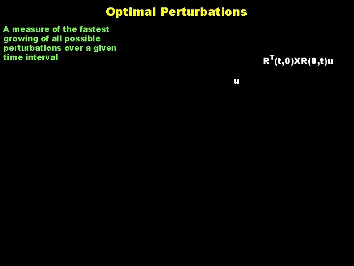
Optimal Perturbations A measure of the fastest growing of all possible perturbations over a given time interval RT(t, 0)XR(0, t)u u

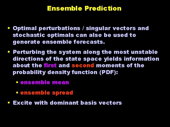
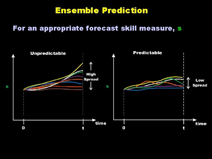
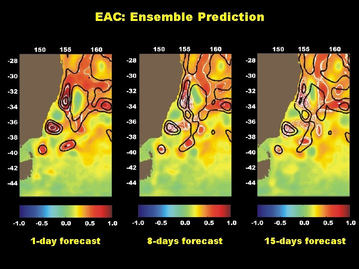
Ensemble Prediction • Optimal perturbations / singular vectors and stochastic optimals can also be used to generate ensemble forecasts. • Perturbing the system along the most unstable directions of the state space yields information about the first and second moments of the probability density function (PDF): § ensemble mean § ensemble spread • Excite with dominant basis vectors

Ensemble Prediction For an appropriate forecast skill measure, s

East Australia Current (EAC) Example

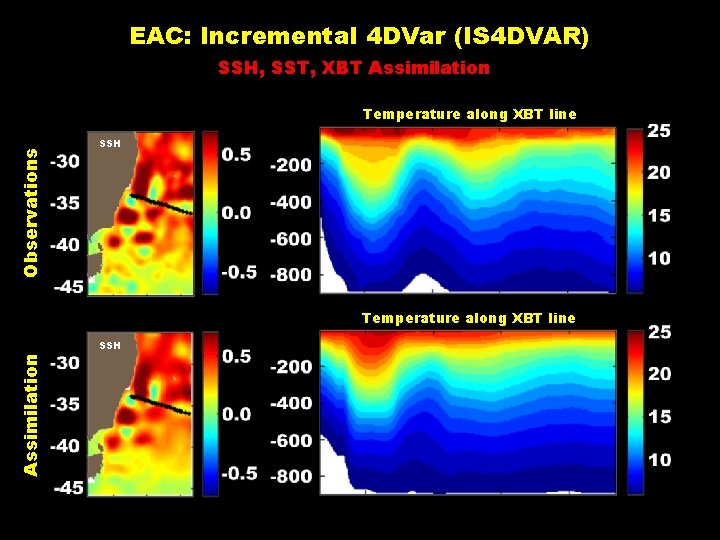
EAC: Incremental 4 DVar (IS 4 DVAR) SSH, SST, XBT Assimilation Observations Temperature along XBT line SSH Temperature along XBT line Assimilation SSH

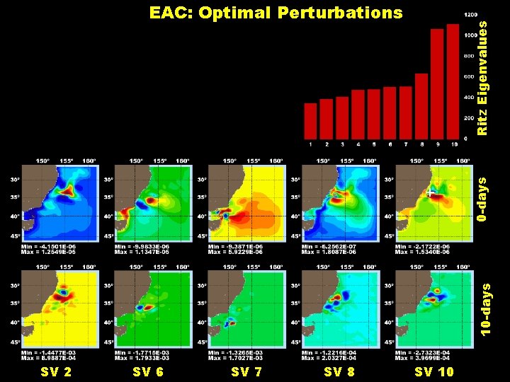
10 -days + 0 -days Ritz Eigenvalues EAC: Optimal Perturbations SV 2 SV 6 SV 7 SV 8 SV 10

EAC: Ensemble Prediction 1 -day forecast 8 -days forecast 15 -days forecast

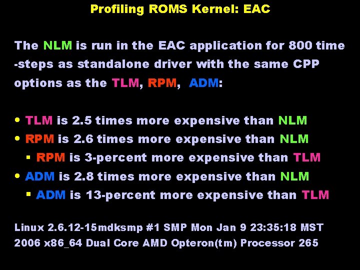
Profiling ROMS Kernel: EAC The NLM is run in the EAC application for 800 time -steps as standalone driver with the same CPP options as the TLM, RPM, ADM: • TLM is 2. 5 times more expensive than NLM • RPM is 2. 6 times more expensive than NLM § RPM is 3 -percent more expensive than TLM • ADM is 2. 8 times more expensive than NLM § ADM is 13 -percent more expensive than TLM Linux 2. 6. 12 -15 mdksmp #1 SMP Mon Jan 9 23: 35: 18 MST 2006 x 86_64 Dual Core AMD Opteron(tm) Processor 265