Robustness for Highdimensional Data Rob HD 2004 Vorau

Robustness for High-dimensional Data Rob. HD 2004, Vorau, May 5 th-8 th 2004 Signal Extraction from Time Series Roland Fried Ursula Gather Universidad Carlos III Universität Dortmund de Madrid, Spain Germany

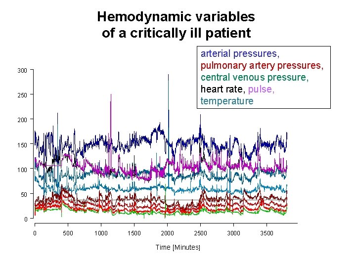
Hemodynamic variables of a critically ill patient arterial pressures, pulmonary artery pressures, central venous pressure, heart rate, pulse, temperature 300 250 200 150 100 50 0 0 500 1000 1500 2000 2500 Time [Minutes] 3000 3500

Goals of Clinical Data Analysis • Intelligent Alarm Systems • Clinical Decision Support • • • Signal extraction Outlier detection / classification Level shift / trend detection Dimension reduction Fast, automatic algorithms Good clinical interpretability

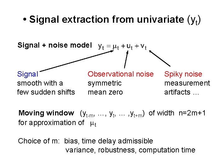
• Signal extraction from univariate (yt) Signal + noise model Signal smooth with a few sudden shifts Observational noise symmetric mean zero Spiky noise measurement artifacts … Moving window (yt-m, …, yt, … , yt+m) of width n=2 m+1 for approximation of Choice of m: bias, time delay admissible variance, robustness, computation time

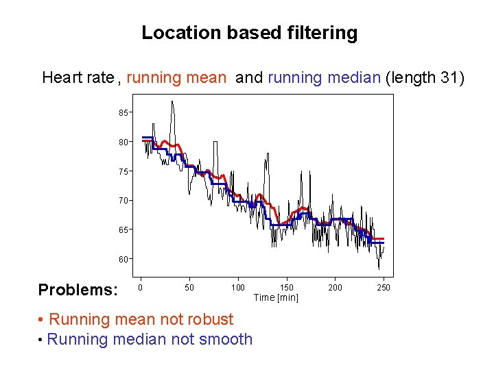
Location based filtering Heart rate , running mean and running median (length 31) 85 80 75 70 65 60 Problems: 0 50 100 • Running mean not robust • Running median not smooth 150 Time [min] 200 250

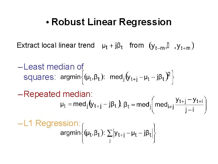
• Robust Linear Regression Extract local linear trend – Least median of squares: – Repeated median: – L 1 Regression: from

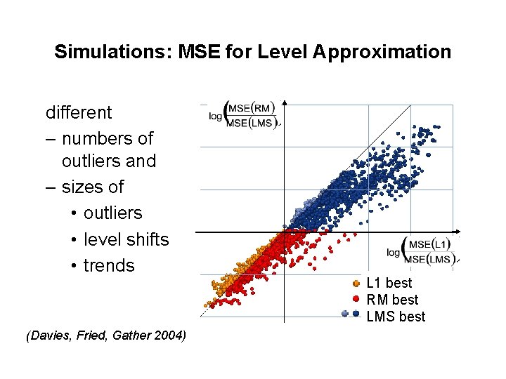
Simulations: MSE for Level Approximation different – numbers of outliers and – sizes of • outliers • level shifts • trends (Davies, Fried, Gather 2004) L 1 best RM best LMS best

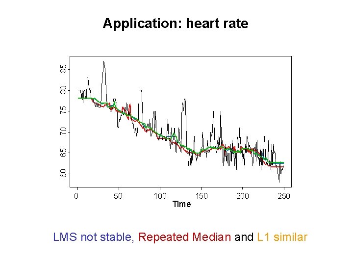
60 65 70 75 80 85 Application: heart rate 0 50 100 Time 150 200 250 LMS not stable, Repeated Median and L 1 similar

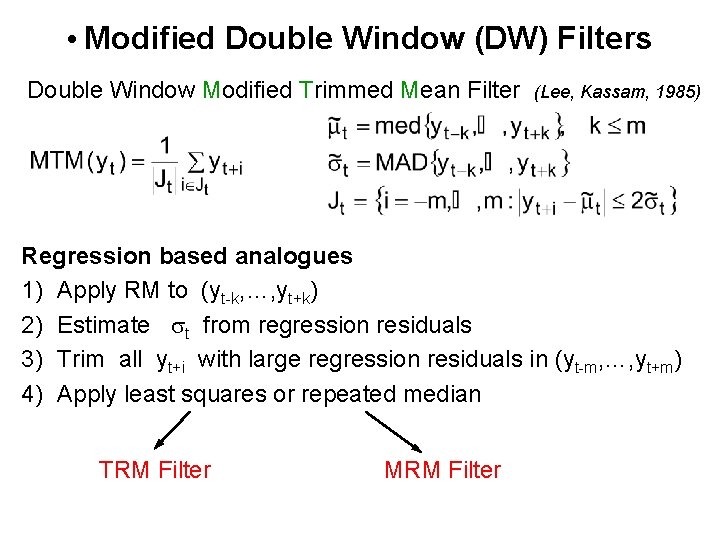
• Modified Double Window (DW) Filters Double Window Modified Trimmed Mean Filter (Lee, Kassam, 1985) Regression based analogues 1) Apply RM to (yt-k, …, yt+k) 2) Estimate st from regression residuals 3) Trim all yt+i with large regression residuals in (yt-m, …, yt+m) 4) Apply least squares or repeated median TRM Filter MRM Filter

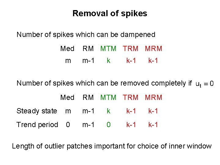
Removal of spikes Number of spikes which can be dampened Med m RM MTM TRM MRM m-1 k k-1 Number of spikes which can be removed completely if Med RM MTM TRM MRM Steady state m m-1 k k-1 Trend period 0 m-1 0 k-1 Length of outlier patches important for choice of inner window

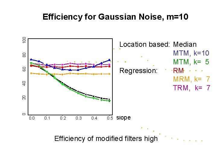
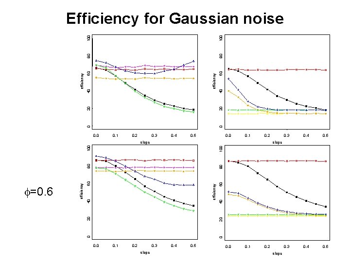
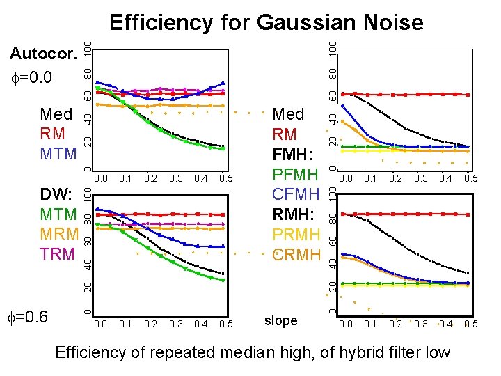
100 Efficiency for Gaussian Noise, m=10 0 20 40 60 80 Location based: Median MTM, k=10 MTM, k= 5 Regression: RM MRM, k= 7 TRM, k= 7 0. 0 0. 1 0. 2 0. 3 0. 4 0. 5 slope Efficiency of modified filters high

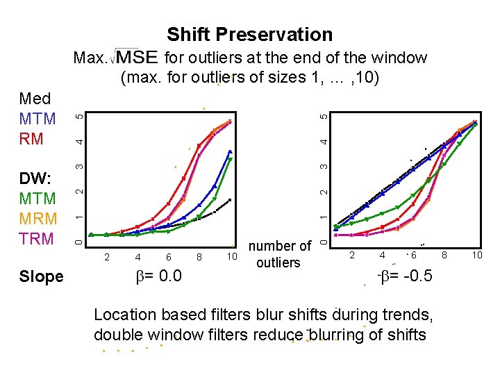
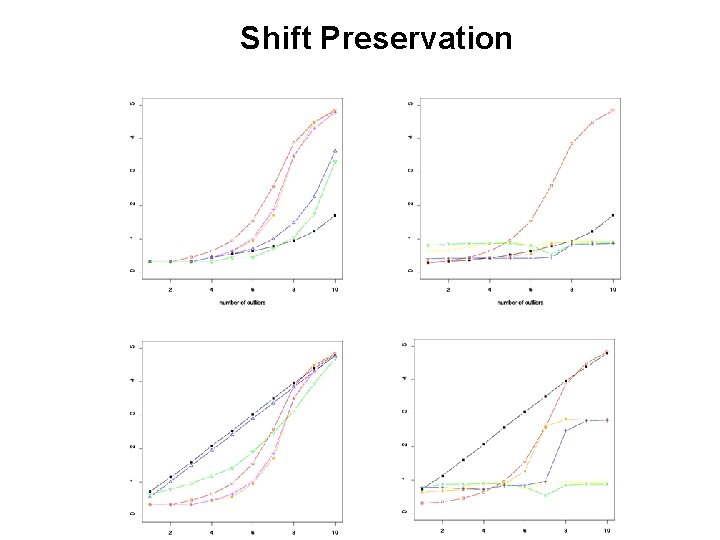
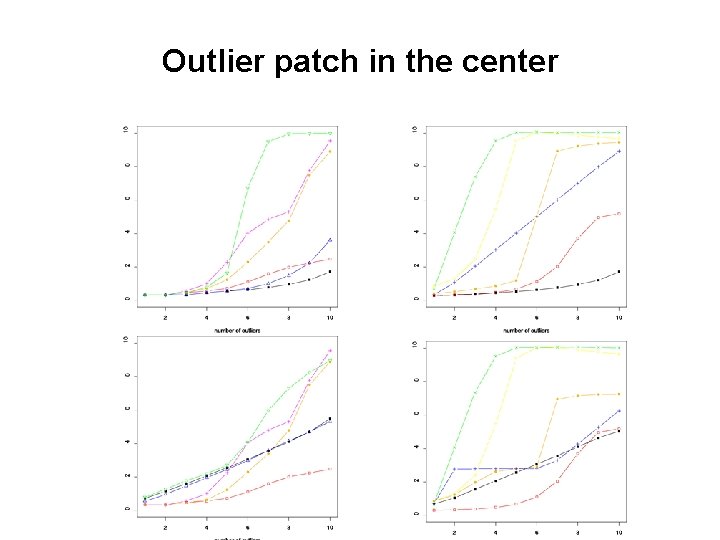
Shift Preservation 5 4 3 3 2 2 1 1 2 Slope 4 6 b= 0. 0 8 10 number of outliers 0 4 DW: MTM MRM TRM for outliers at the end of the window (max. for outliers of sizes 1, … , 10) 5 Med MTM RM 0 Max. 2 4 6 b= -0. 5 Location based filters blur shifts during trends, double window filters reduce blurring of shifts 8 10

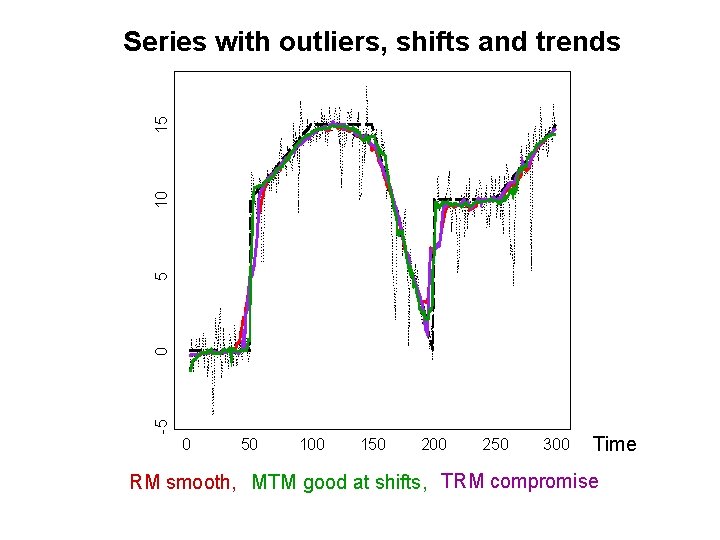
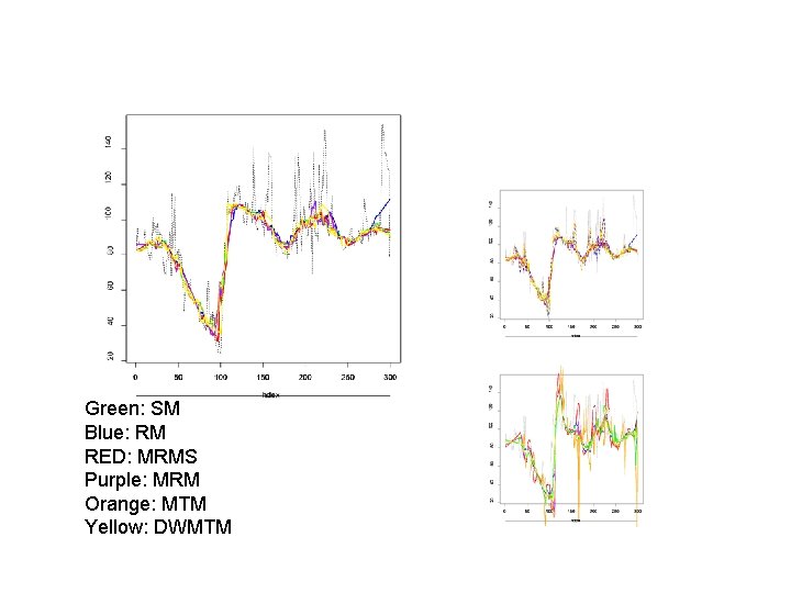
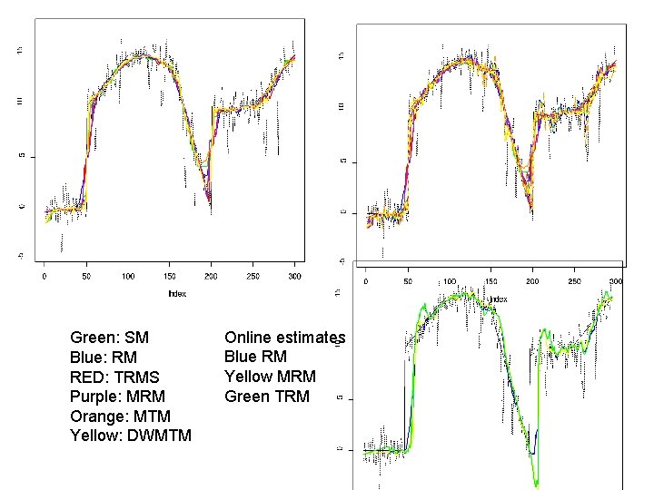
-5 0 5 10 15 Series with outliers, shifts and trends 0 50 100 150 200 250 300 Time RM smooth, MTM good at shifts, TRM compromise

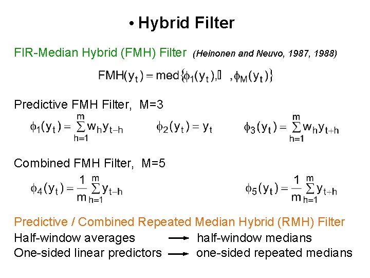
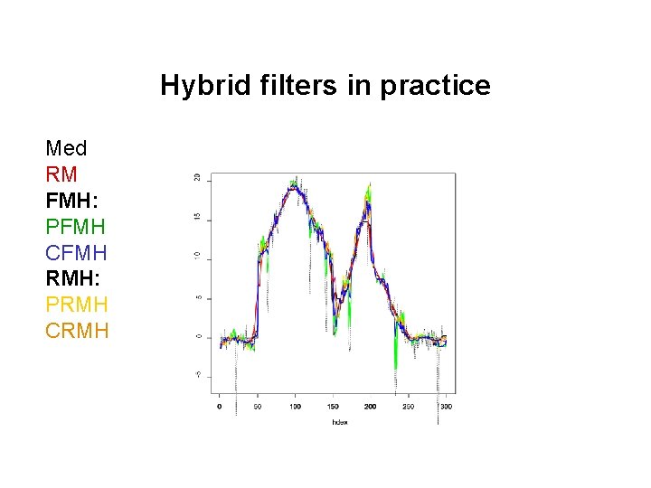
• Hybrid Filter FIR-Median Hybrid (FMH) Filter (Heinonen and Neuvo, 1987, 1988) Predictive FMH Filter, M=3 Combined FMH Filter, M=5 Predictive / Combined Repeated Median Hybrid (RMH) Filter Half-window averages half-window medians One-sided linear predictors one-sided repeated medians

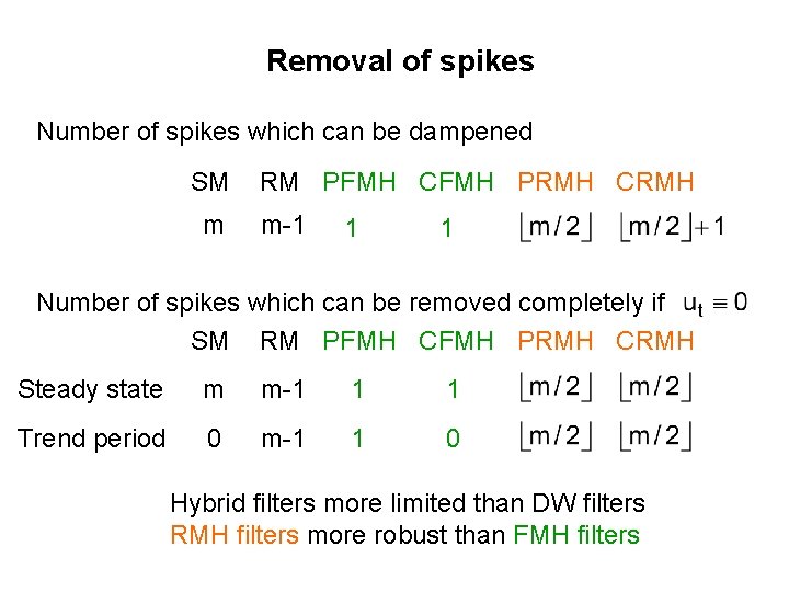
Removal of spikes Number of spikes which can be dampened SM m RM PFMH CFMH PRMH CRMH m-1 1 1 Number of spikes which can be removed completely if SM RM PFMH CFMH PRMH CRMH Steady state m m-1 1 1 Trend period 0 m-1 1 0 Hybrid filters more limited than DW filters RMH filters more robust than FMH filters

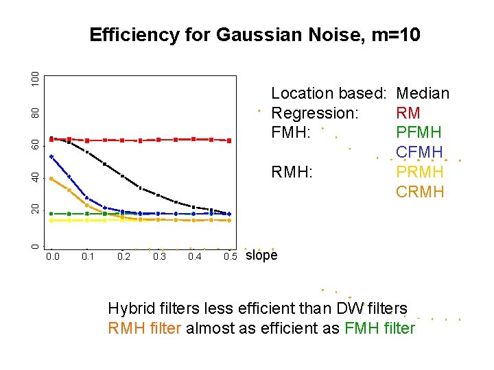
100 Efficiency for Gaussian Noise, m=10 0 20 40 60 80 Location based: Median Regression: RM FMH: PFMH CFMH RMH: PRMH CRMH 0. 0 0. 1 0. 2 0. 3 0. 4 0. 5 slope Hybrid filters less efficient than DW filters RMH filter almost as efficient as FMH filter

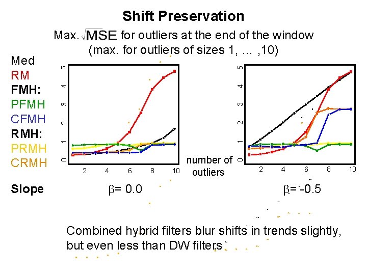
Shift Preservation Slope 5 3 4 4 2 3 2 2 4 6 b= 0. 0 8 10 number of outliers 0 1 1 0 Med RM FMH: PFMH CFMH RMH: PRMH CRMH for outliers at the end of the window (max. for outliers of sizes 1, … , 10) 5 Max. 2 4 6 8 b= -0. 5 Combined hybrid filters blur shifts in trends slightly, but even less than DW filters 10

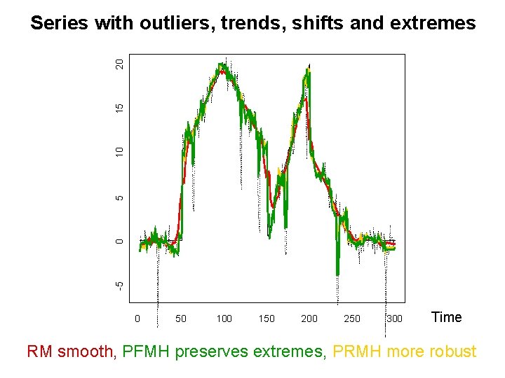
-5 0 5 10 15 20 Series with outliers, trends, shifts and extremes 0 50 100 150 200 250 300 Time RM smooth, PFMH preserves extremes, PRMH more robust

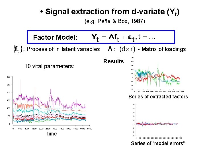
• Signal extraction from d-variate (Yt) (e. g. Peña & Box, 1987) Factor Model: Process of r latent variables 10 vital parameters: - Matrix of loadings Results Series of extracted factors time Series of “model errors’’

Conclusion • Extraction of time-varying mean from contaminated time series by robust regression • LMS very robust, but slow and unstable Repeated median robust, fast and stable • Double window and hybrid filters improve preservation of shifts and extremes • Adaptive window width selection Full online version Multivariate signal extraction

References Bernholt, T. , Fried, R. (2003). Computing the update of the repeated median regression line in linear time. Information Processing Letters 88, 111 -117. Davies, P. L. , Fried, R. , Gather, U. (2004). Robust signal extraction for on-line monitoring data. J. Statistical Planning and Inference, 122, 65 -78. Fried, R. (2004). Robust filtering of time series with trends. J. Nonparametric Statistics, to appear. Fried, R. , Bernholt, T. , Gather, U. (2004). Repeated median and hybrid filters. Technical Report 10/2004, SFB 475, University of Dortmund, Germany. Gather, U. , Fried, R. (2004 a). Robust scale estimation for local linear temporal trends. Tatra Mountains Mathematical Publications, 26, 87 -101. Gather, U. , Fried, R. (2004 b). Methods and algorithms for robust filtering. Proceedings of COMPSTAT 2004, to appear.

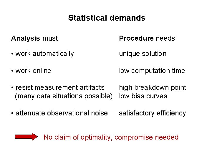
Statistical demands Analysis must Procedure needs • work automatically unique solution • work online low computation time • resist measurement artifacts high breakdown point (many data situations possible) low bias curves • attenuate observational noise satisfactory efficiency No claim of optimality, compromise needed

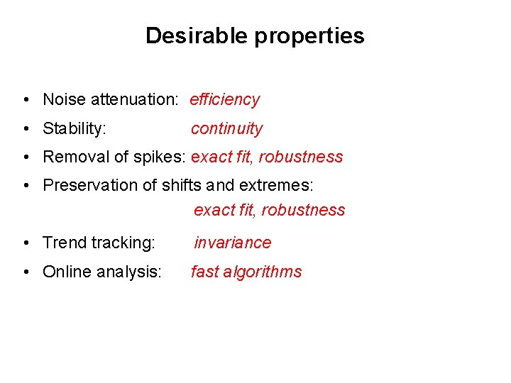
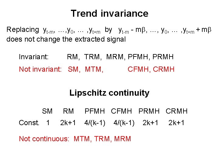
Desirable properties • Noise attenuation: efficiency • Stability: continuity • Removal of spikes: exact fit, robustness • Preservation of shifts and extremes: exact fit, robustness • Trend tracking: invariance • Online analysis: fast algorithms

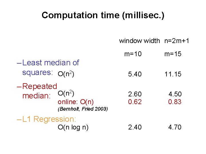
Computation time (millisec. ) window width n=2 m+1 – Least median of squares: O(n 2) – Repeated 2) O(n median: online: O(n) m=10 m=15 5. 40 11. 15 2. 60 0. 62 4. 50 0. 83 2. 40 4. 70 (Bernholt, Fried 2003) – L 1 Regression: O(n log n)

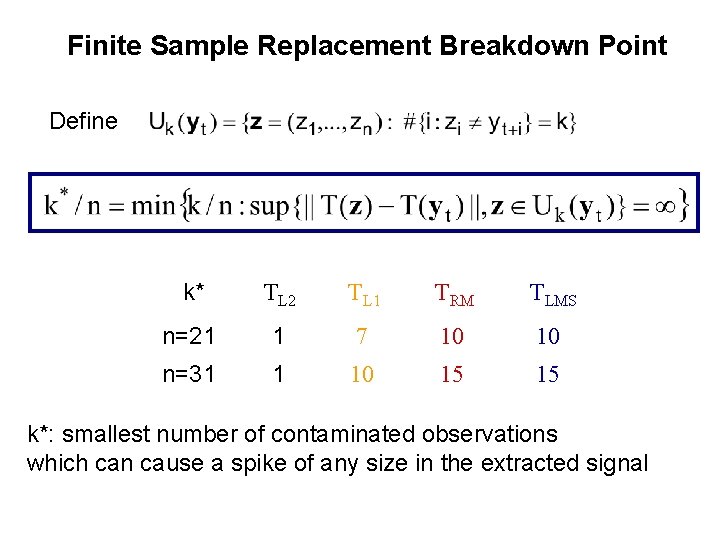
Finite Sample Replacement Breakdown Point Define k* TL 2 TL 1 TRM TLMS n=21 1 7 10 10 n=31 1 10 15 15 k*: smallest number of contaminated observations which can cause a spike of any size in the extracted signal

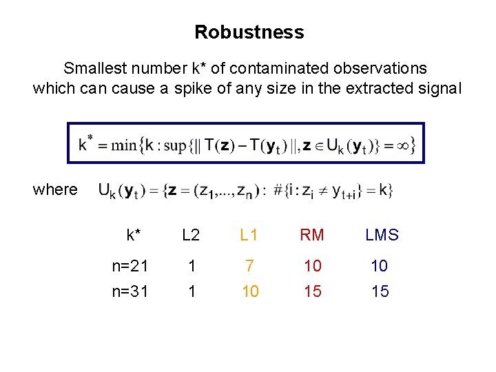
Robustness Smallest number k* of contaminated observations which can cause a spike of any size in the extracted signal where k* L 2 L 1 RM LMS n=21 1 7 10 10 n=31 1 10 15 15

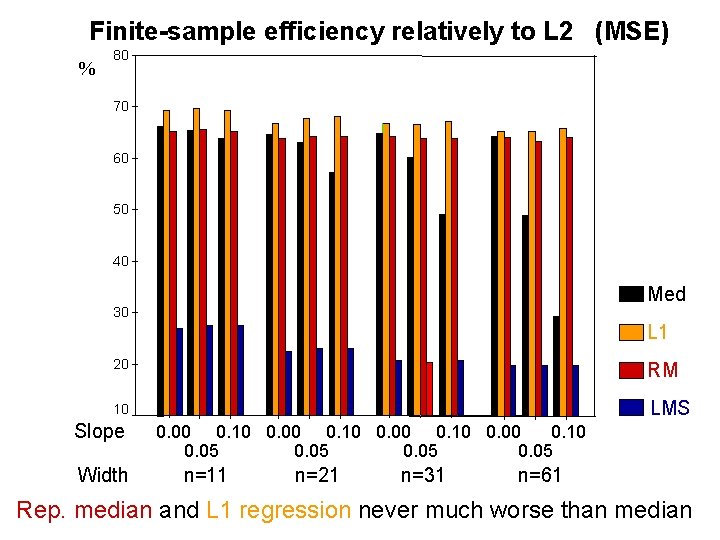
Finite-sample efficiency relatively to L 2 (MSE) % 80 70 60 50 40 Med 30 L 1 20 RM 10 LMS Slope Width 0. 00 0. 10 0. 05 n=11 n=21 n=31 n=61 Rep. median and L 1 regression never much worse than median

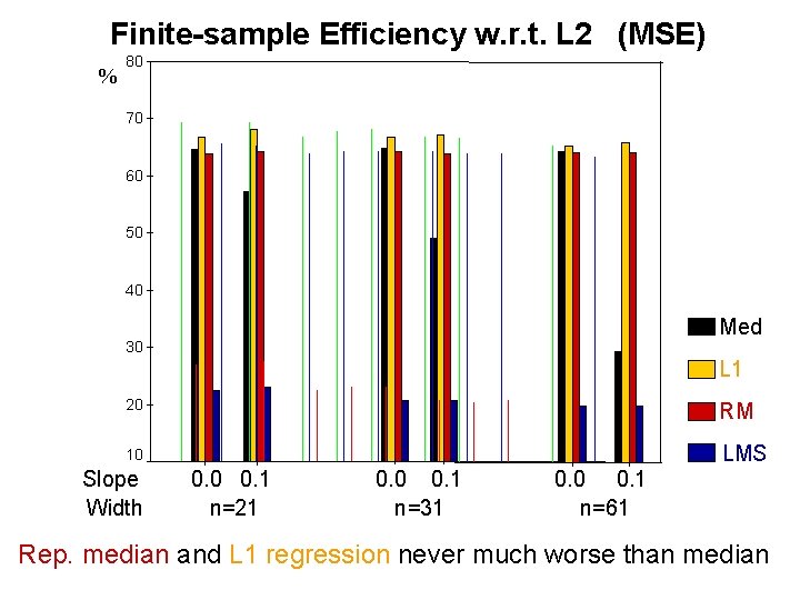
Finite-sample Efficiency w. r. t. L 2 (MSE) % 80 70 60 50 40 Med 30 L 1 20 RM 10 LMS Slope Width 0. 0 0. 1 n=21 0. 0 0. 1 n=31 0. 0 0. 1 n=61 Rep. median and L 1 regression never much worse than median

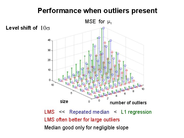
Performance when outliers present MSE for Level shift of size number of outliers LMS << Repeated median < L 1 regression LMS often better for large outliers Median good only for negligible slope

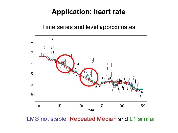
Application: heart rate Time series and level approximates LMS not stable, Repeated Median and L 1 similar

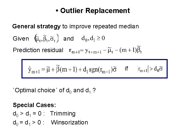
• Outlier Replacement General strategy to improve repeated median Given and Prediction residual if `Optimal choice´ of d 0 and d 1 ? Special Cases: d 0 > d 1 = 0 : Trimming d 0 = d 1 > 0 : Winsorization

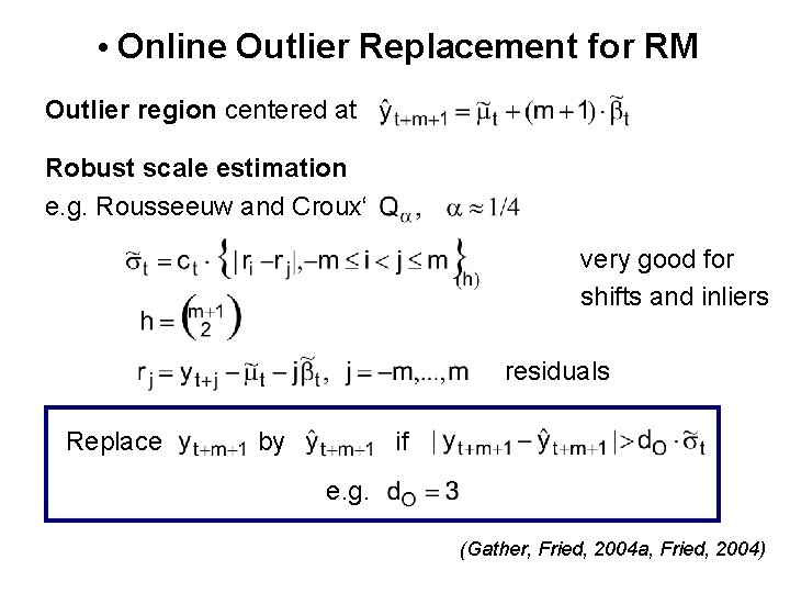
• Online Outlier Replacement for RM Outlier region centered at Robust scale estimation e. g. Rousseeuw and Croux‘ very good for shifts and inliers residuals Replace by if e. g. (Gather, Fried, 2004 a, Fried, 2004)

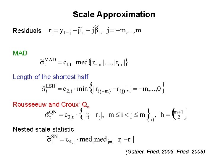
Scale Approximation Residuals MAD Length of the shortest half Rousseeuw and Croux‘ Qa Nested scale statistic (Gather, Fried, 2003)

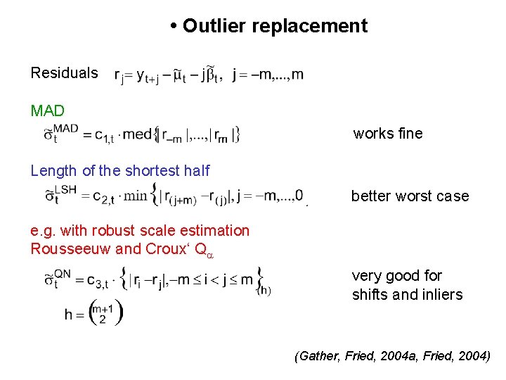
• Outlier replacement Residuals MAD works fine Length of the shortest half better worst case e. g. with robust scale estimation Rousseeuw and Croux‘ Qa very good for shifts and inliers (Gather, Fried, 2004 a, Fried, 2004)

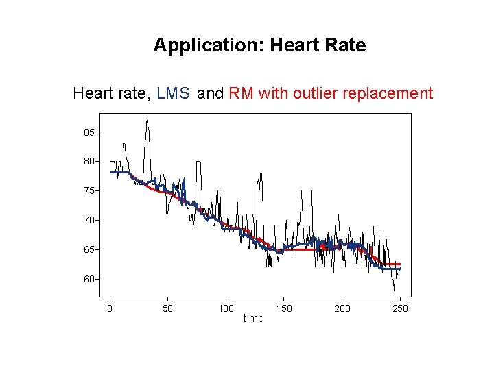
Application: Heart Rate Heart rate , LMS and RM with outlier replacement 85 80 75 70 65 60 0 50 100 time 150 200 250

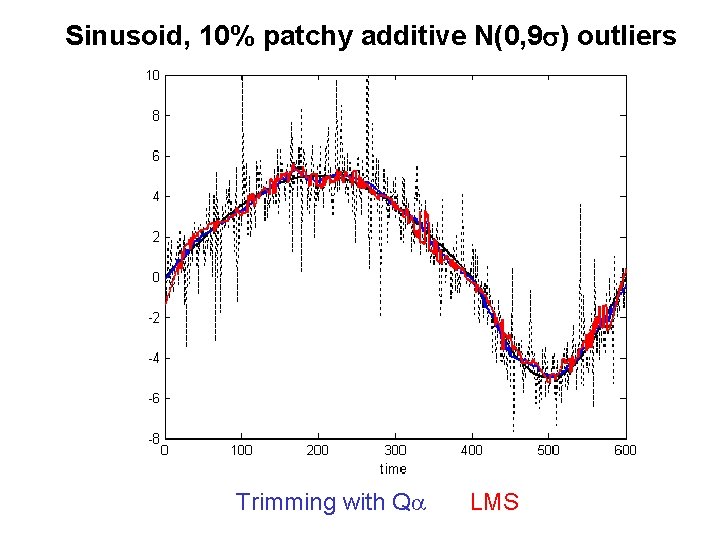
Sinusoid, 10% patchy additive N(0, 9 s) outliers Trimming with Qa LMS

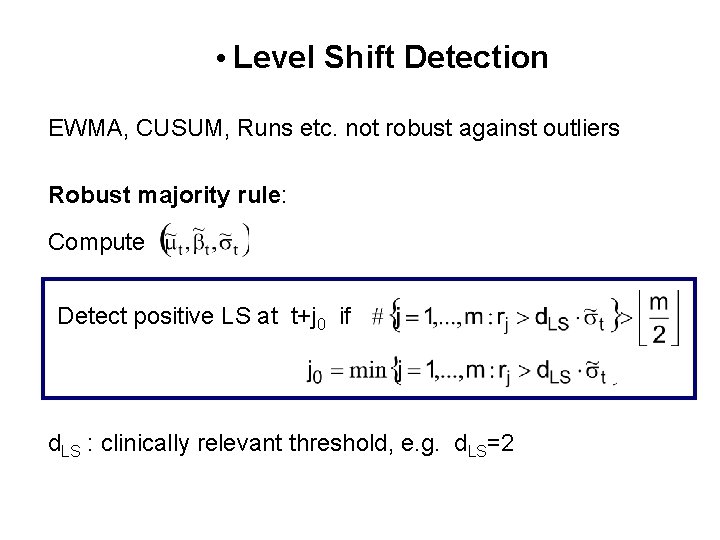
• Level Shift Detection EWMA, CUSUM, Runs etc. not robust against outliers Robust majority rule: Compute Detect positive LS at t+j 0 if d. LS : clinically relevant threshold, e. g. d. LS=2

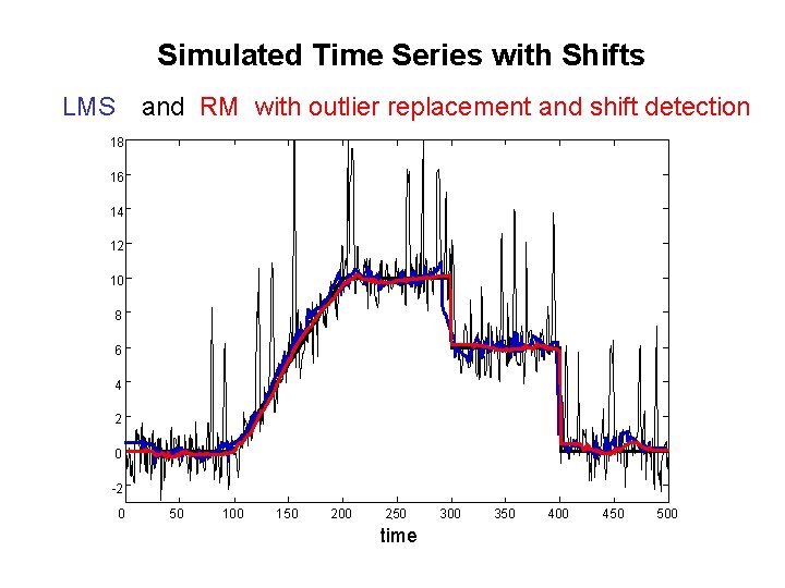
Simulated Time Series with Shifts LMS and RM with outlier replacement and shift detection 18 16 14 12 10 8 6 4 2 0 -2 0 50 100 150 200 250 time 300 350 400 450 500

Trend invariance Replacing yt-m, …, y 0, … , yt+m by yt-m - mb, …, y 0, … , yt+m + mb does not change the extracted signal Invariant: RM, TRM, MRM, PFMH, PRMH Not invariant: SM, MTM, CFMH, CRMH Lipschitz continuity SM Const. 1 RM 2 k+1 PFMH CFMH PRMH CRMH 4/(k-1) Not continuous: MTM, TRM, MRM 2 k+1

100 60 20 40 efficiency 60 40 0 0 20 efficiency 80 80 100 Efficiency for Gaussian noise 0. 0 0. 1 0. 2 0. 3 0. 4 0. 0 0. 5 0. 1 0. 2 slope 0. 4 0. 5 0. 3 0. 4 0. 5 60 40 20 20 40 efficiency 60 80 80 100 slope 0 0 efficiency f=0. 6 0. 3 0. 0 0. 1 0. 2 0. 3 slope 0. 4 0. 5 0. 0 0. 1 0. 2 slope

100 80 80 0. 5 0. 0 0. 1 0. 2 0. 3 0. 4 0. 5 80 60 40 20 0 0. 1 0. 2 0. 3 0. 4 0. 5 0. 0 0. 1 0. 2 0. 3 0. 4 0. 5 slope 0 20 40 0 f=0. 6 0. 0 100 0. 4 80 0. 3 60 0. 2 100 0. 1 20 DW: MTM MRM TRM 0. 0 Med RM FMH: PFMH CFMH RMH: PRMH CRMH 40 40 20 0 Med RM MTM 60 60 Autocor. f=0. 0 100 Efficiency for Gaussian Noise Efficiency of repeated median high, of hybrid filter low

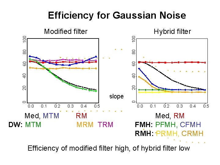
Efficiency for Gaussian Noise Hybrid filter 20 20 40 40 60 60 80 80 100 Modified filter 0 0 slope 0. 0 0. 1 0. 2 Med, MTM DW: MTM 0. 3 0. 4 0. 5 RM MRM TRM 0. 0 0. 1 0. 2 0. 3 0. 4 0. 5 Med, RM FMH: PFMH, CFMH RMH: PRMH, CRMH Efficiency of modified filter high, of hybrid filter low

Shift Preservation

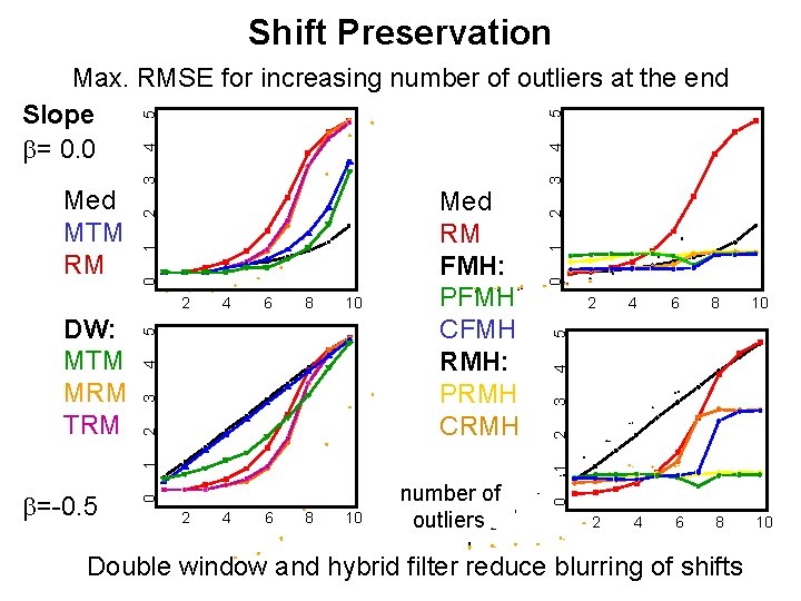
Shift Preservation 4 3 2 2 1 0 4 6 8 2 4 6 8 10 1 2 4 6 8 10 number of outliers 0 0 b=-0. 5 2 5 10 4 8 3 6 1 DW: MTM MRM TRM 4 5 2 Med RM FMH: PFMH CFMH RMH: PRMH CRMH 2 1 0 Med MTM RM 2 3 3 4 4 5 5 Max. RMSE for increasing number of outliers at the end Slope b= 0. 0 Double window and hybrid filter reduce blurring of shifts 10

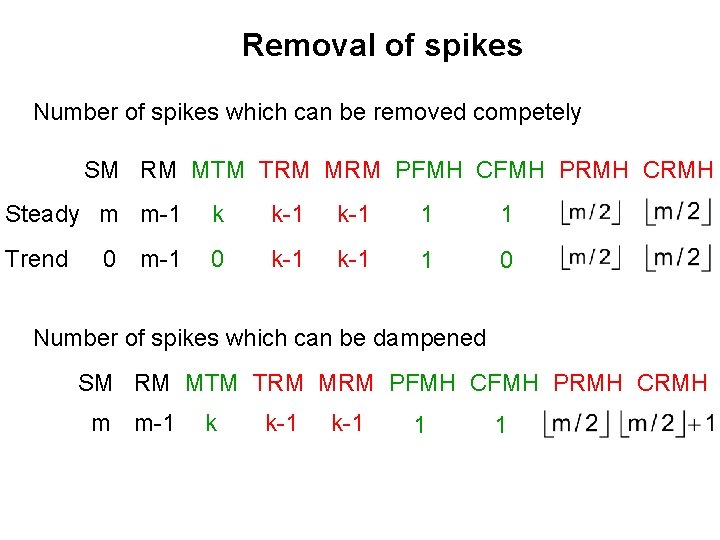
Removal of spikes Number of spikes which can be removed competely SM RM MTM TRM MRM PFMH CFMH PRMH CRMH Steady m m-1 k k-1 1 1 Trend 0 k-1 1 0 0 m-1 Number of spikes which can be dampened SM RM MTM TRM MRM PFMH CFMH PRMH CRMH m m-1 k k-1 1 1

Outlier patch in the center

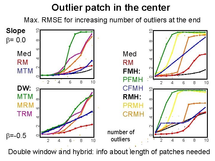
Outlier patch in the center 10 8 6 4 2 0 6 8 10 2 4 6 8 10 10 4 2 4 6 8 10 number of outliers 0 2 4 0 b=-0. 5 2 8 10 6 8 4 6 10 4 2 DW: MTM MRM TRM 2 Med RM FMH: PFMH CFMH RMH: PRMH CRMH 6 8 8 6 4 0 Med RM MTM 2 Slope b= 0. 0 10 Max. RMSE for increasing number of outliers at the end Double window and hybrid: info about length of patches needed

Green: SM Blue: RM RED: MRMS Purple: MRM Orange: MTM Yellow: DWMTM

Green: SM Blue: RM RED: TRMS Purple: MRM Orange: MTM Yellow: DWMTM Online estimates Blue RM Yellow MRM Green TRM

Hybrid filters in practice Med RM FMH: PFMH CFMH RMH: PRMH CRMH

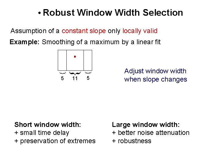
• Robust Window Width Selection Assumption of a constant slope only locally valid 5 11 { { { Example: Smoothing of a maximum by a linear fit 5 Short window width: + small time delay + preservation of extremes Adjust window width when slope changes Large window width: + better noise attenuation + robustness

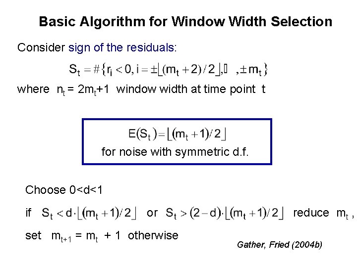
Basic Algorithm for Window Width Selection Consider sign of the residuals: where nt = 2 mt+1 window width at time point t for noise with symmetric d. f. Choose 0<d<1 if or set mt+1 = mt + 1 otherwise reduce mt , Gather, Fried (2004 b)

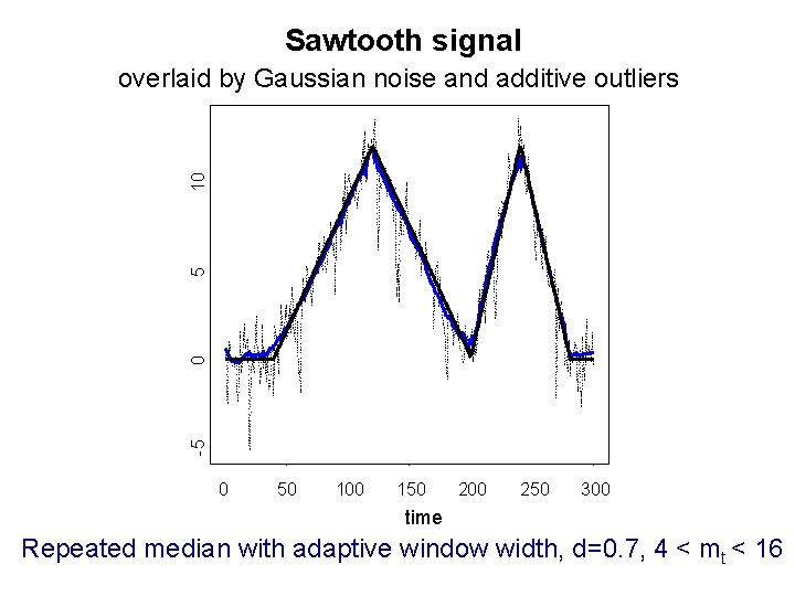
Sawtooth signal -5 0 5 10 overlaid by Gaussian noise and additive outliers 0 50 100 150 200 250 300 time Repeated median with adaptive window width, d=0. 7, 4 < mt < 16

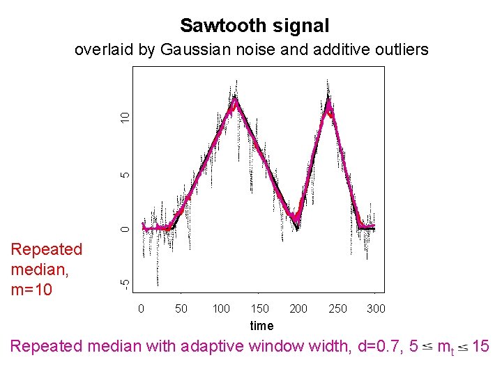
Sawtooth signal Repeated median, m=10 -5 0 5 10 overlaid by Gaussian noise and additive outliers 0 50 100 150 200 250 300 time Repeated median with adaptive window width, d=0. 7, 5 mt 15

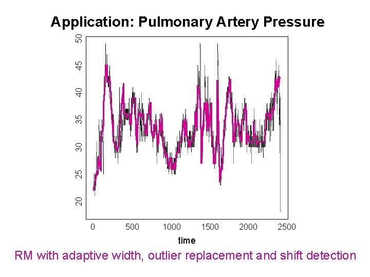
20 25 30 35 40 45 50 Application: Pulmonary Artery Pressure 0 500 1000 1500 2000 2500 time RM with adaptive width, outlier replacement and shift detection

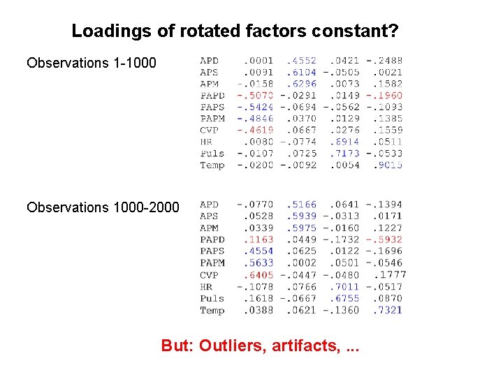
Loadings of rotated factors constant? Observations 1 -1000 Observations 1000 -2000 But: Outliers, artifacts, . . .

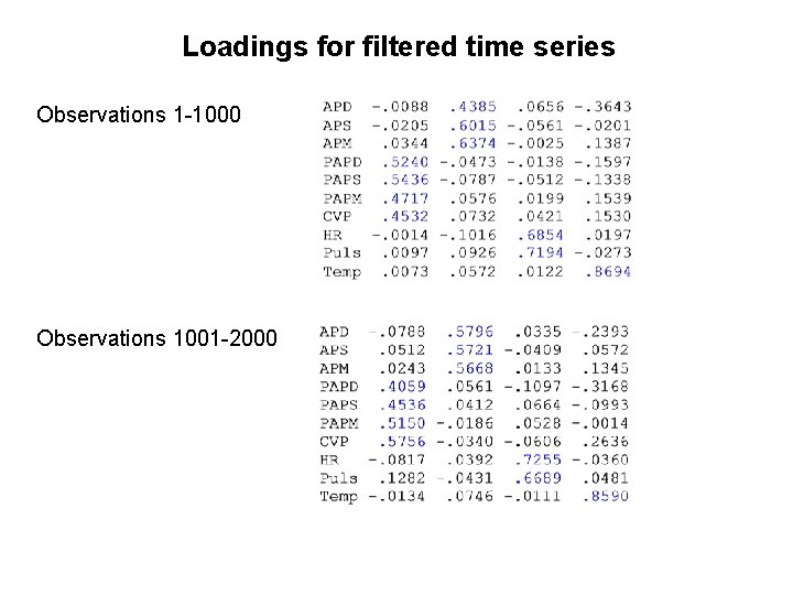
Loadings for filtered time series Observations 1 -1000 Observations 1001 -2000