Robust Visual Motion Analysis PiecewiseSmooth Optical Flow Ming

Robust Visual Motion Analysis: Piecewise-Smooth Optical Flow Ming Ye Electrical Engineering, University of Washington mingye@u. washington. edu

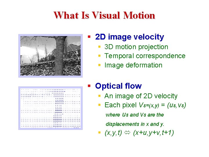
What Is Visual Motion § 2 D image velocity § 3 D motion projection § Temporal correspondence § Image deformation § Optical flow § An image of 2 D velocity § Each pixel Vs=(x, y) = (us, vs) where us and vs are the displacements in x and y. § (x, y, t) (x+u, y+v, t+1)

Structure From Motion Rigid scene + camera translation Estimated horizontal motion Depth map

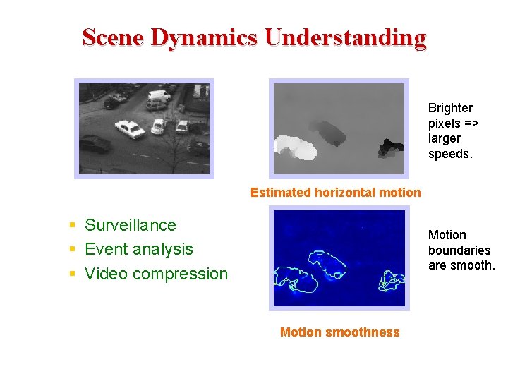
Scene Dynamics Understanding Brighter pixels => larger speeds. Estimated horizontal motion § Surveillance § Event analysis § Video compression Motion boundaries are smooth. Motion smoothness

Target Detection and Tracking A tiny airplane --- only observable by its distinct motion Tracking results

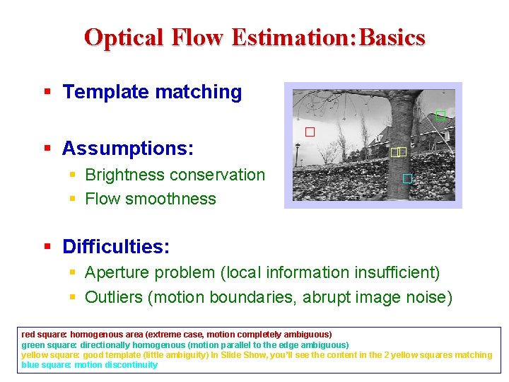
Optical Flow Estimation: Basics § Template matching § Assumptions: § Brightness conservation § Flow smoothness § Difficulties: § Aperture problem (local information insufficient) § Outliers (motion boundaries, abrupt image noise) red square: homogenous area (extreme case, motion completely ambiguous) green square: directionally homogenous (motion parallel to the edge ambiguous) yellow square: good template (little ambiguity) In Slide Show, you’ll see the content in the 2 yellow squares matching blue square: motion discontinuity

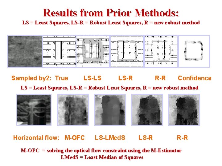
Results from Prior Methods: LS = Least Squares, LS-R = Robust Least Squares, R = new robust method Sampled by 2: True LS-LS LS-R R-R Confidence LS = Least Squares, LS-R = Robust Least Squares, R = new robust method Horizontal flow: M-OFC LS-LMed. S LS-R R-R M-OFC = solving the optical flow constraint using the M-Estimator LMed. S = Least Median of Squares

Estimating Piecewise-Smooth Optical Flow with Global Matching and Graduated Optimization A Bayesian Approach

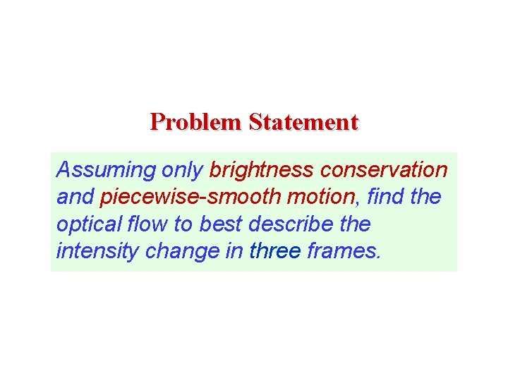
Problem Statement Assuming only brightness conservation and piecewise-smooth motion, find the optical flow to best describe the intensity change in three frames.

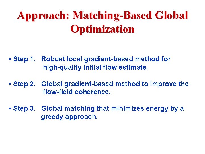
Approach: Matching-Based Global Optimization • Step 1. Robust local gradient-based method for high-quality initial flow estimate. • Step 2. Global gradient-based method to improve the flow-field coherence. • Step 3. Global matching that minimizes energy by a greedy approach.

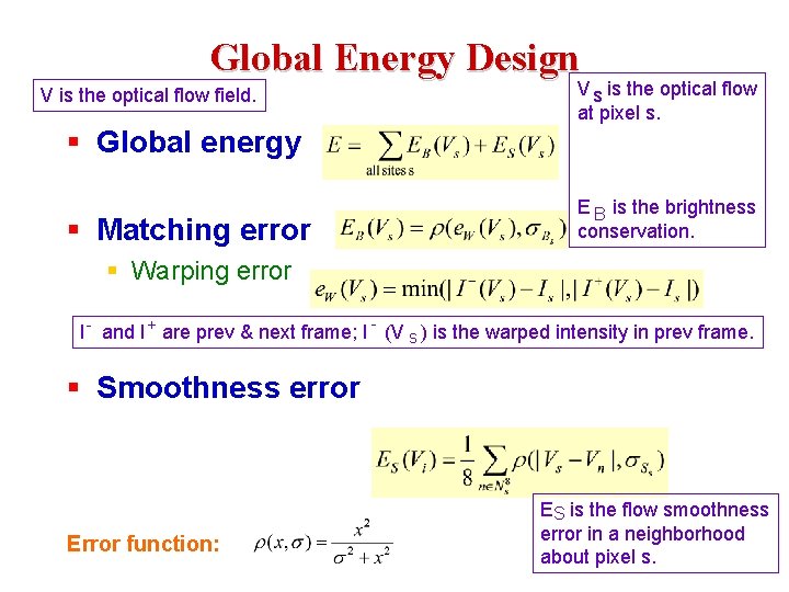
Global Energy Design V s is the optical flow at pixel s. V is the optical flow field. § Global energy E B is the brightness conservation. § Matching error § Warping error - I - and I + are prev & next frame; I (V s ) is the warped intensity in prev frame. § Smoothness error Error function: ES is the flow smoothness error in a neighborhood about pixel s.

Step 1: Gradient-Based Local Regression • A crude flow estimate is assumed available (and has been compensated for) • A robust gradient-based local regression is used to compute the incremental flow V. • The dominant translational motion in the neighborhood of each pixel is computed by solving a set of flow equations using a least-median-of-squares criterion.

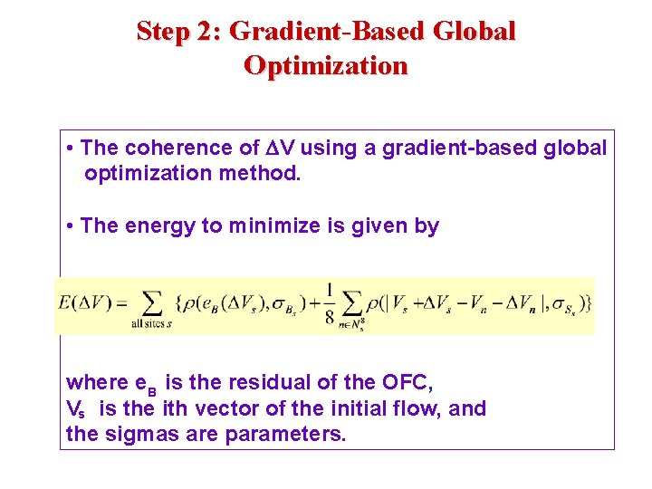
Step 2: Gradient-Based Global Optimization • The coherence of V using a gradient-based global optimization method. • The energy to minimize is given by where e. B is the residual of the OFC, Vs is the ith vector of the initial flow, and the sigmas are parameters.

Step 3: Global Matching • The new flow estimate still exhibits gross errors at motion boundaries and other places with poor gradient estimates. • This error is reduced by solving the matching-based formulation equation through greedy propagation. • The energy is calculated for all pixels. • Then each pixel is visited, examining whether a trial estimate from the candidates in its neighborhood is better (lower energy). If so, this becomes the new estimate for that pixel. This is repeated iteratively.

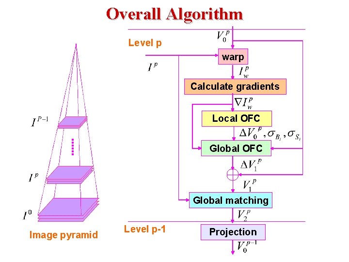
Overall Algorithm Level p warp Calculate gradients Local OFC Global matching Image pyramid Level p-1 Projection

Advantages § Best of Everything § Local OFC § High-quality initial flow estimates § Robust local scale estimates § Global OFC § Improve flow smoothness § Global Matching § The optimal formulation § Correct errors caused by poor gradient quality and hierarchical process § Results: fast convergence, high accuracy, simultaneous motion boundary detection

Experiments • Experiments were run on several standard test videos. • Estimates of optical flow were made for the middle frame of every three. • The results were compared with the Black and Anandan algorithm.

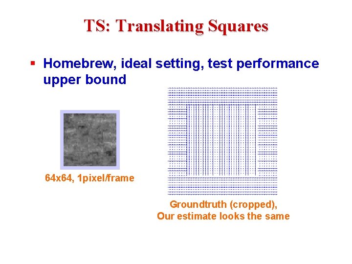
TS: Translating Squares § Homebrew, ideal setting, test performance upper bound 64 x 64, 1 pixel/frame Groundtruth (cropped), Our estimate looks the same

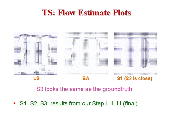
TS: Flow Estimate Plots LS BA S 1 (S 2 is close) S 3 looks the same as the groundtruth. § S 1, S 2, S 3: results from our Step I, III (final)

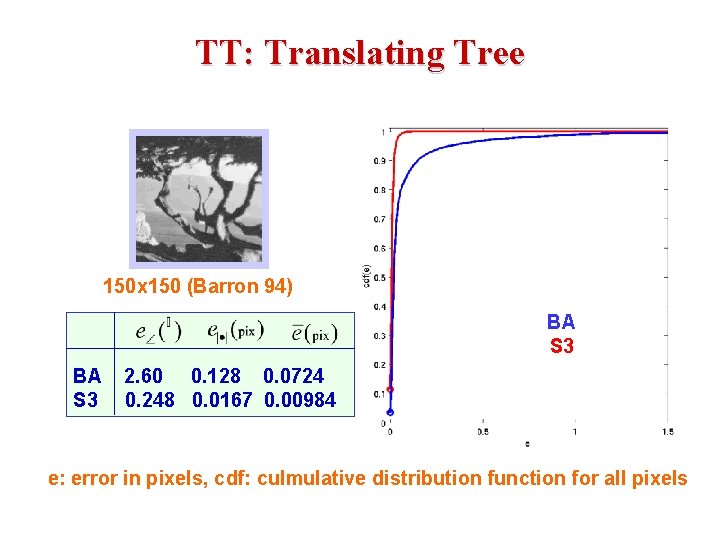
TT: Translating Tree 150 x 150 (Barron 94) BA S 3 2. 60 0. 128 0. 0724 0. 248 0. 0167 0. 00984 e: error in pixels, cdf: culmulative distribution function for all pixels

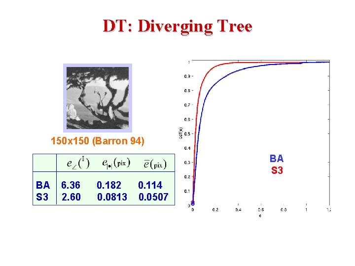
DT: Diverging Tree 150 x 150 (Barron 94) BA S 3 6. 36 2. 60 0. 182 0. 0813 0. 114 0. 0507

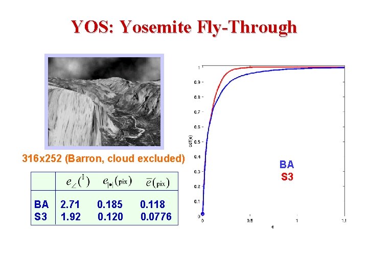
YOS: Yosemite Fly-Through 316 x 252 (Barron, cloud excluded) BA S 3 2. 71 1. 92 0. 185 0. 120 0. 118 0. 0776 BA S 3

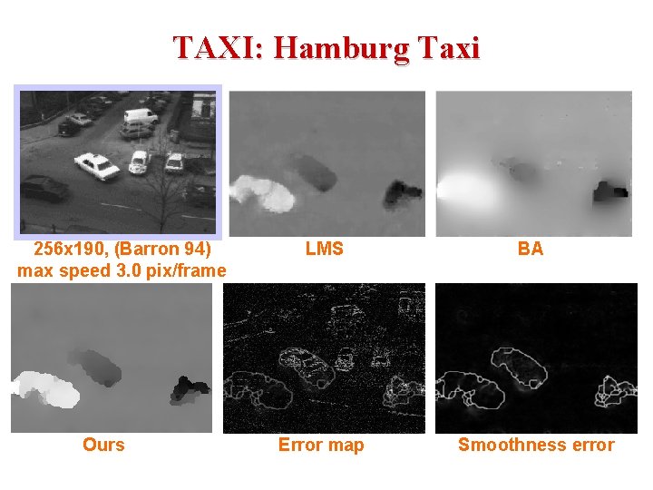
TAXI: Hamburg Taxi 256 x 190, (Barron 94) max speed 3. 0 pix/frame Ours LMS BA Error map Smoothness error

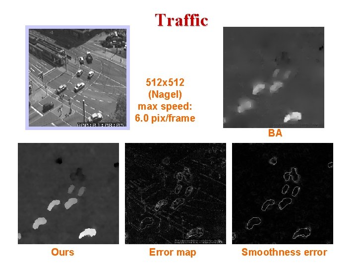
Traffic 512 x 512 (Nagel) max speed: 6. 0 pix/frame BA Ours Error map Smoothness error

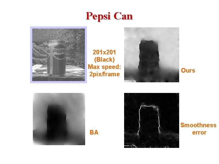
Pepsi Can 201 x 201 (Black) Max speed: 2 pix/frame BA Ours Smoothness error

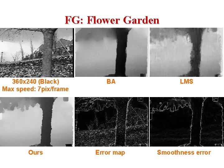
FG: Flower Garden 360 x 240 (Black) Max speed: 7 pix/frame BA Ours Error map LMS Smoothness error

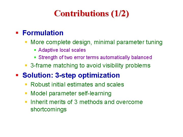
Contributions (1/2) § Formulation § More complete design, minimal parameter tuning § Adaptive local scales § Strength of two error terms automatically balanced § 3 -frame matching to avoid visibility problems § Solution: 3 -step optimization § Robust initial estimates and scales § Model parameter self-learning § Inherit merits of 3 methods and overcome shortcomings

Contributions (2/2) § Results § High accuracy § Fast convergence § By product: motion boundaries § Significance § Foundation for higher-level (model-based) visual motion analysis § Methodology applicable to other low-level vision problems