ROBUST STATISTICS INTRODUCTION Robust statistics provides an alternative

ROBUST STATISTICS

INTRODUCTION • Robust statistics provides an alternative approach to classical statistical methods. The motivation is to produce estimators that are not excessively affected by small departures from model assumptions. These departures may include departures from an assumed sample distribution or data departuring from the rest of the data (i. e. outliers). • The goal is to produce statistical procedures which still behave fairly well under deviations from the assumed model.

INTRODUCTION • Mosteller and Tukey define two types of robustness: • resistance means that changing a small part, even by a large amount, of the data does not cause a large change in the estimate • robustness of efficiency means that the statistic has high efficiency in a variety of situations rather than in any one situation. Efficiency means that the estimate is close to optimal estimate given that we know what distribution that the data comes from. A useful measure of efficiency is: Efficiency = (lowest variance feasible)/ (actual variance) • Many statistics have one of these properties. However, it can be difficult to find statistics that are both resistant and have robustness of efficiency.


MEAN VS MEDIAN •

ROBUST MEASURE OF VARIABILITY •

ROBUST MEASURE OF CORRELATION • The Pearson correlation coefficient is an optimal estimator for Gaussian data. However, it is not resistant and it does not have robustness of efficiency. • The percentage bend correlation estimator, discussed in Shoemaker and Hettmansperger and also by Wilcox, is both resistant and robust of efficiency. • When the underlying data are bivariate normal, ρpb gives essentially the same values as Pearson’s ρ. In general, ρpb is more robust to slight changes in the data than ρ.
 where we")
Example • We use a simple dataset from Wright and London (2009) where we are interested whether the length and heat of a chile are related. The length was measured in centimeters, the heat on a scale from 0 (“for sissys”) to 11 (“nuclear”). head(chile) name length heat 1 Afric 5. 00 5. 0 2 Aji 7. 50 7. 0 3 Aji_A 11. 43 7. 5 4 Aji_C 3. 81 9. 0 5 Aji_F 6. 00 2. 0 6 Aji_L 6. 35 7. 0 library(vioplot) attach(chile) plot(length, heat, xlim=c(0, 32), ylim=c(0, 11)) vioplot(length, col="red", at=0, horizontal=TRUE, add=TRUE) vioplot(heat, col="blue", at=0, horizontal=FALSE, add=TRUE with(chile, pbcor(length, heat)) Call: pbcor(x = length, y = heat) Robust correlation coefficient: -0. 3785 Test statistic: -3. 7251 p-value: 0. 00035)

ROBUST MEASURE OF CORRELATION • A second robust correlation measure is the Winsorized correlation ρw, which requires the specification of the amount of Winsorization. • The computation is simple: it uses Person’s correlation formula applied on the Winsorized data.

Example • In a study on the effect of consuming alcohol, the number hangover symptoms were measured for two independent groups, with each subject consuming alcohol and being measured on three different occasions. One group consisted of sons of alcoholics and the other one was a control group. Here we are interested in the Winsorized correlations across the three time points for the participants in the alcoholic group: library(WRS 2) library(reshape) hangctr <- subset(hangover, subset = group == "alcoholic") hangctr symptoms group time id 61 0 alcoholic 1 21 62 0 alcoholic 1 22 63 0 alcoholic 1 23 64 0 alcoholic 1 24 65 0 alcoholic 1 25 66 0 alcoholic 1 26 67 0 alcoholic 1 27 68 0 alcoholic 1 28 hangwide <- cast(hangctr, id ~ time, value = "symptoms")[, -1] hangwide 1 2 3 Cast a molten data frame into the reshaped or aggregated form you want 1 0 2 1 2 0 0 0 3 0 7 3 4 0 0 0 5 0 4 3
 Call: winall(x = hangwide) Robust correlation matrix: 1 2 3 1 1. 0000")
winall(hangwide) Call: winall(x = hangwide) Robust correlation matrix: 1 2 3 1 1. 0000 0. 2651 0. 4875 2 0. 2651 1. 0000 0. 6791 3 0. 4875 0. 6791 1. 0000 p-values: 1 2 3 1 NA 0. 27046 0. 03935 2 0. 27046 NA 0. 00284 3 0. 03935 0. 00284 NA

ORDER STATISTICS AND ROBUSTNESS • Ordered statistics and their functions are usually somewhat robust (e. g. median, MAD, IQR), but not all ordered statistics are robust (e. g. X(1), X(n), R=X(n) X(1).
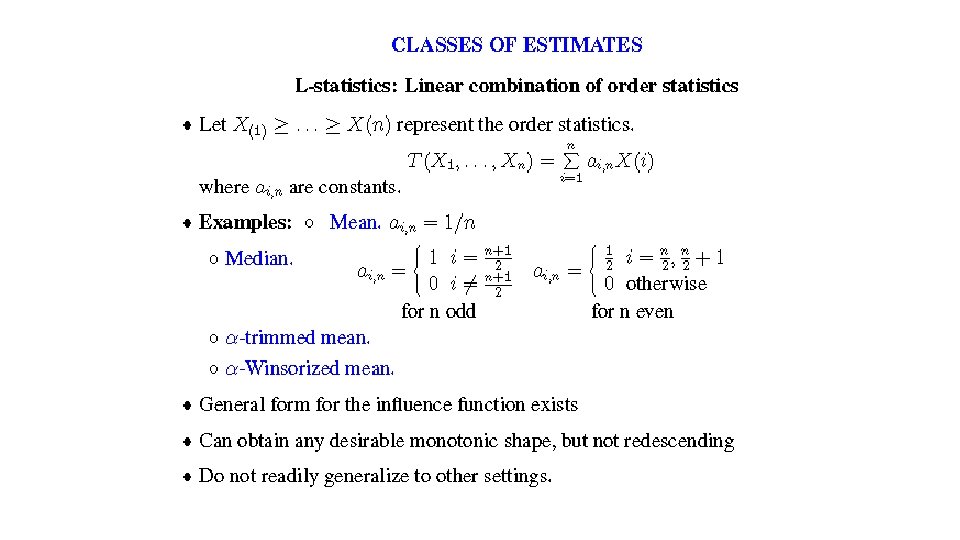

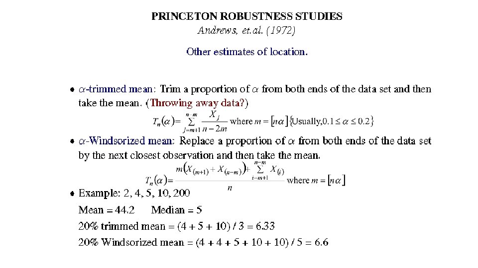
• REMARK: mean, α-trimmed mean and α-Winsorized mean, median are particular cases of L-statistics • L-statistics: linear combination of order statistics. • Classical estimators are highly influenced by the outlier • Robust estimate computed from all observations is comparable with the classical estimate applied to non-outlying data • How to compare robust estimators?
 sensitivity curve (SC) •")
(Standardized) sensitivity curve (SC) •
 • Data �� 10={�� 1, …, �� 10} are the natural")
Sensitivity curve (example) • Data �� 10={�� 1, …, �� 10} are the natural logs of the annual incomes of 10 people. 9. 52 9. 68 10. 16 9. 96 10. 08 9. 99 10. 47 9. 91 9. 92 15. 21 . y 9 consist of the 9 ‘regular’ observations
 breakdown point • Given data set with nobs. • If replace m")
(Finite sample) breakdown point • Given data set with nobs. • If replace m of obs. by any outliers and estimator stays in a bounded set, but doesn't when we replace (m+1), the breakdown point of the estimator at that data set is m/n. • breakdown point of the mean= 0
 breakdown pointof the median • �� is even • �� is odd")
(Finite sample) breakdown pointof the median • �� is even • �� is odd
 •")
INFLUENCE FUNCTION (Hampel, 1974) •
")
INFLUENCE FUNCTION (IF)
")
PLOT OF THE INFLUENCE FUNCTION AT N(0, 1)

SC and IF • IF : small fraction ε of identical outliers • SC : fraction of contamination is 1/��

M-ESTIMATORS •

M-ESTIMATORS •

M-ESTIMATORS •

M-ESTIMATORS •

M-ESTIMATOR • When an estimator is robust, it may be inferred that the influence of any single observation is insufficient to yield any significant offset. There are several constraints that a robust M-estimator should meet: 1. The first is of course to have a bounded influence function. 2. The second is naturally the requirement of the robust estimator to be unique.
")
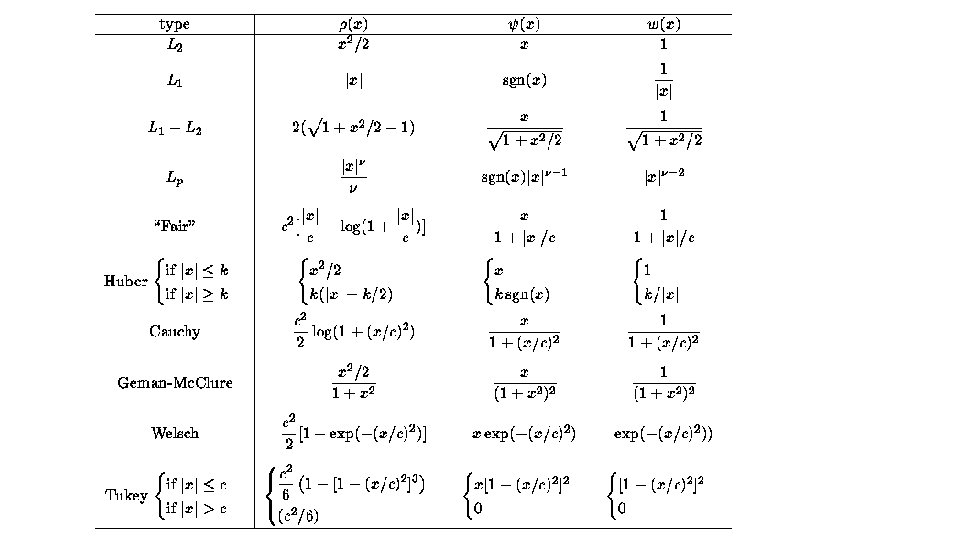
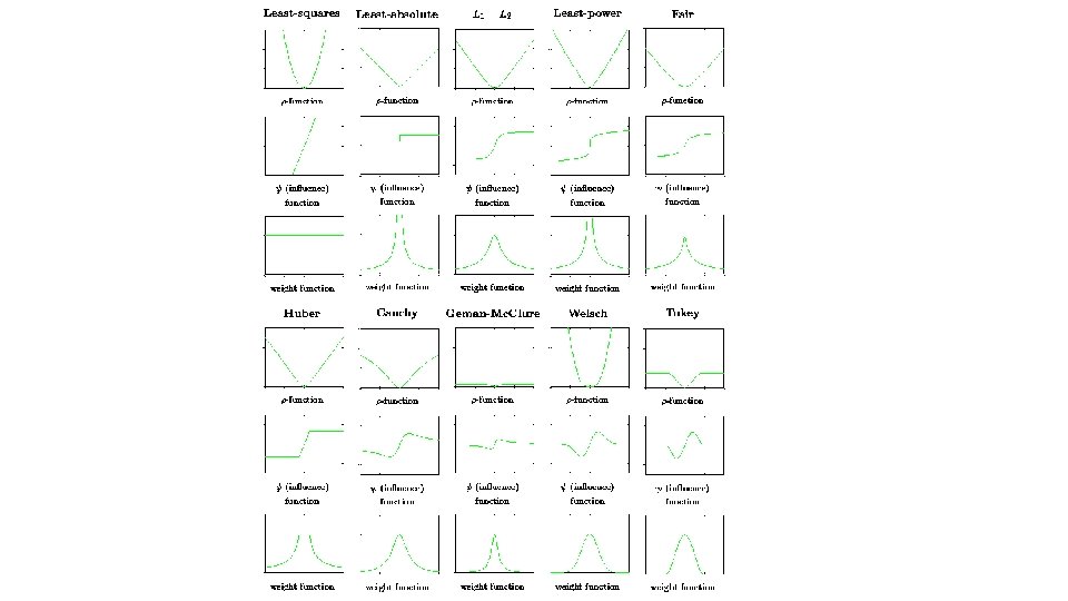
Briefly we give a few indications of these functions: • L 2 (least-squares) estimators are not robust because their influence function is not bounded. • L 1 (absolute value) estimators are not stable because the function |x| is not strictly convex in x. Indeed, the second derivative at x=0 is unbounded, and an indeterminant solution may result. • L 1 L 2 estimators reduce the influence of large errors, but they still have an influence because the influence function has no cut off point.
 = x 2, and the")
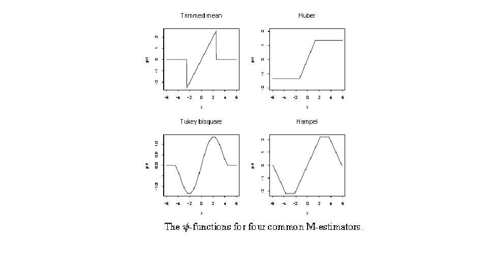
EXAMPLES OF M-ESTIMATORS • The mean corresponds to ρ(x) = x 2, and the median to ρ(x) = |x|. (For even n any median will solve the problem. ) The function corresponds to metric trimming and large outliers have no influence at all. The function is known as metric Winsorizing 2 and brings in extreme observations to μ±c.

EXAMPLES OF M-ESTIMATORS • The corresponding −log f is and corresponds to a density with a Gaussian center and doubleexponential tails. This estimator is due to Huber.
![EXAMPLES OF M-ESTIMATORS • Tukey’s biweight has where [ ]+ denotes the positive part](http://slidetodoc.com/presentation_image_h/8d7a3d6425bdbc499a9f7576142c4061/image-35.jpg "EXAMPLES OF M-ESTIMATORS • Tukey’s biweight has where [ ]+ denotes the positive part")
EXAMPLES OF M-ESTIMATORS • Tukey’s biweight has where [ ]+ denotes the positive part of. This implements ‘soft’ trimming. The value R = 4. 685 gives 95% efficiency at the normal. • Hampel’s ψ has several linear pieces, for example, with a = 2. 2 s, b = 3. 7 s, c = 5. 9 s.

ROBUST REGRESSION • Robust estimation procedures dampen the influence of outlying cases, as compared to ordinary LSE, in an effort to provide a better fit for the majority of cases. • LEAST ABSOLUTE RESIDUALS (LAR) REGRESSION: Estimates the regression coefficients by minimizing the sum of absolute deviations of Y observations from their means: Since absolute deviations rather than squared ones are involved, LAR places less emphasis on outlying observations than does the method of LS. Residuals ordinarily will not sum to 0. Solution for estimated coefficients may not be unique.
 ROBUST REGRESSION: It uses weighted least")
ROBUST REGRESSION • ITERATIVELY REWEIGHTED LEAST SQUARES (IRLS) ROBUST REGRESSION: It uses weighted least squares procedure. This regression uses weights based on how far outlying a case is, as measured by the residual for that case. The weights are revised with each iteration until a robust fit has been obtained.
 REGRESSION: • Other robust regression methods:")
ROBUST REGRESSION • LEAST MEDIAN OF SQUARES (LMS) REGRESSION: • Other robust regression methods: Some involve trimming extreme squared deviations before applying LSE, others are based on ranks. Many of the robust regression procedures require intensive computing.

EXAMPLE • This data set gives n = 24 observations about the annual numbers of telephone calls made (calls, in millions of calls) in Belgium in the last two digits of the year (year); see Rousseeuw and Leroy (1987), and Venables and Ripley (2002). As it can be noted in Figure there are several outliers in the y-direction in the late 1960 s.
 attach(phones)")
• Let us start the analysis with the classical OLS fit. library(MASS) attach(phones) plot(year, calls) fit. ols <- lm(calls~year) summary(fit. ols, cor=F) Residuals: Min 1 Q Median 3 Q Max -78. 97 -33. 52 -12. 04 23. 38 124. 20 Coefficients: Estimate Std. Error t value Pr(>|t|) (Intercept) -260. 059 102. 607 -2. 535 0. 0189 * year 5. 041 1. 658 3. 041 0. 0060 ** --Signif. codes: 0 ‘***’ 0. 001 ‘**’ 0. 01 ‘*’ 0. 05 ‘. ’ 0. 1 ‘ ’ 1 Residual standard error: 56. 22 on 22 degrees of freedom Multiple R-squared: 0. 2959, Adjusted R-squared: 0. 2639 F-statistic: 9. 247 on 1 and 22 DF, p-value: 0. 005998
 par(mfrow=c(1, 4)) plot(fit. ols, 1: 2) plot(fit. ols, 4) hmat. p <-")
abline(fit. ols$coef) par(mfrow=c(1, 4)) plot(fit. ols, 1: 2) plot(fit. ols, 4) hmat. p <- hat(model. matrix(fit. ols)) h. phone <- hat(hmat. p) cook. d <- cooks. distance(fit. ols) plot(h. phone/(1 -h. phone), cook. d, xlab="h/(1 -h)", ylab="Cook distance")

• In order to take into account of observations related to high values of the residuals, i. e. the outliers in the late 1960 s, consider a robust regression based on Huber-type estimates: fit. hub <- rlm(calls~year, maxit=50) fit. hub 2 <- rlm(calls~year, scale. est="proposal 2") summary(fit. hub, cor=F) Residuals: Min 1 Q Median -18. 314 -5. 953 -1. 681 3 Q Max 26. 460 173. 769 Coefficients: Value Std. Error t value (Intercept) -102. 6222 year 2. 0414 26. 6082 -3. 8568 0. 4299 4. 7480 Residual standard error: 9. 032 on 22 degrees of freedom summary(fit. hub 2, cor=F) Residuals: Min 1 Q Median -68. 15 -29. 46 -11. 52 3 Q Max 22. 74 132. 67 Coefficients: Value (Intercept) -227. 9250 year 4. 4530 Std. Error t value 101. 8740 -2. 2373 1. 6461 2. 7052 Residual standard error: 57. 25 on 22 degrees of freedom
, cor=F) Residuals: Min 1 Q Median 3 Q Max -1.")
> summary(rlm(calls~year, psi=psi. bisquare), cor=F) Residuals: Min 1 Q Median 3 Q Max -1. 6585 -0. 4143 0. 2837 39. 0866 188. 5376 Coefficients: Value Std. Error t value (Intercept) -52. 3025 2. 7530 -18. 9985 year 1. 0980 0. 0445 24. 6846 Residual standard error: 1. 654 on 22 degrees of freedom

• From the results and also from THE PREVIOUS PLOT, we note that there are some differences with the OLS estimates, in particular this is true for the Huber-type estimator with MAD. • Consider again some classic diagnostic plots about the robust fit: the plot of the observed values versus the fitted values, the plot of the residuals versus the fitted values, the normal QQ-plot of the residuals and the fit weights of the robust estimator. Note that there are some observations with low Huber-type weights which were not identified by the classical Cook’s statistics.
- Slides: 45