Robust Kernel Density Estimation by Scaling and Projection

Robust Kernel Density Estimation by Scaling and Projection in Hilbert Space Presented by: Nacer Khalil

Table of content 1. Introduction 1. Definition of robustness 2. Robust Kernel Density Estimation 2. 3. 4. 5. Nonparametric Contamination Models Scaled project Kernel Density Estimator Experiment and conclusion Case study 1

Introduction What is robustness • robustness is the ability of a computer system to cope with errors during execution (wikipedia) • Robustness: – Reliability – Availability – Resilience 2

Introduction What is robustness • Robustness in machine learning is: – The extend to which testing errors is consistent with training errors – The extent to which the performance of the algorithm resists to noise 3

Introduction Robust kernel density estimation • Density Estimation – Parametric – Nonparametric • Non parametric density estimation: – Enables working under more general assumptions, but not robust – Difficulty in making it robust 4

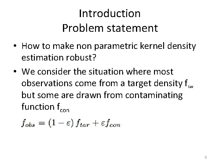
Introduction Problem statement • How to make non parametric kernel density estimation robust? • We consider the situation where most observations come from a target density ftar but some are drawn from contaminating function fcon 5

Introduction Contribution • The authors introduce a new formalism to describe transformations that “decontaminates” fobs • The process of decontamination is: – Scaling: Multiply the KDE by a real number to scale – Shifting: Find closest pdf to the scaled KDE in the L 2 norm 6

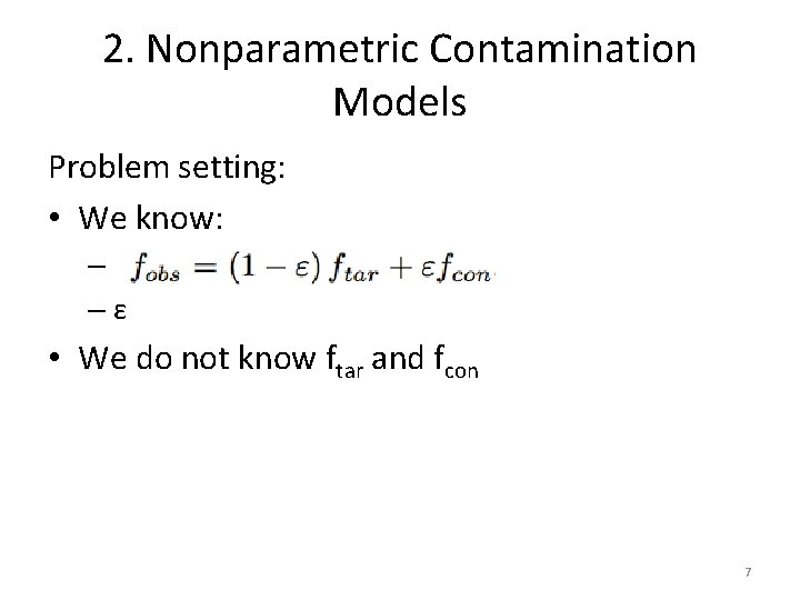
2. Nonparametric Contamination Models Problem setting: • We know: – –ε • We do not know ftar and fcon 7

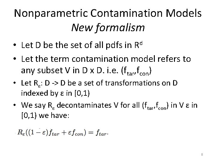
Nonparametric Contamination Models New formalism • Let D be the set of all pdfs in Rd • Let the term contamination model refers to any subset V in D x D. i. e. (ftar, fcon) • Let Rε: D -> D be a set of transformations on D indexed by ε in [0, 1) • We say Rε decontaminates V for all (ftar, fcon) in V ε in [0, 1) we have: 8

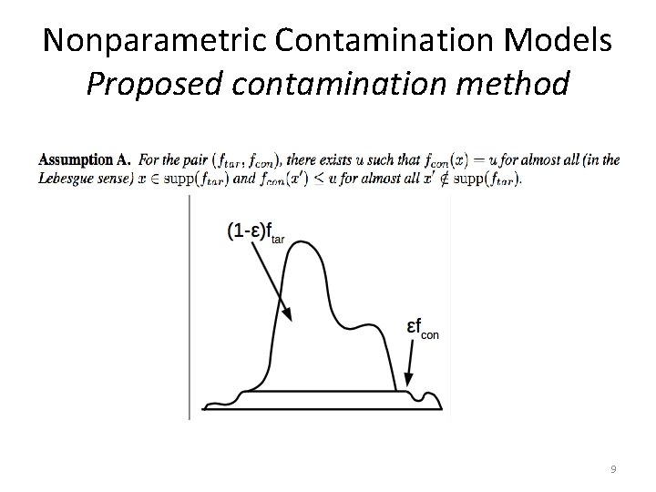
Nonparametric Contamination Models Proposed contamination method 9

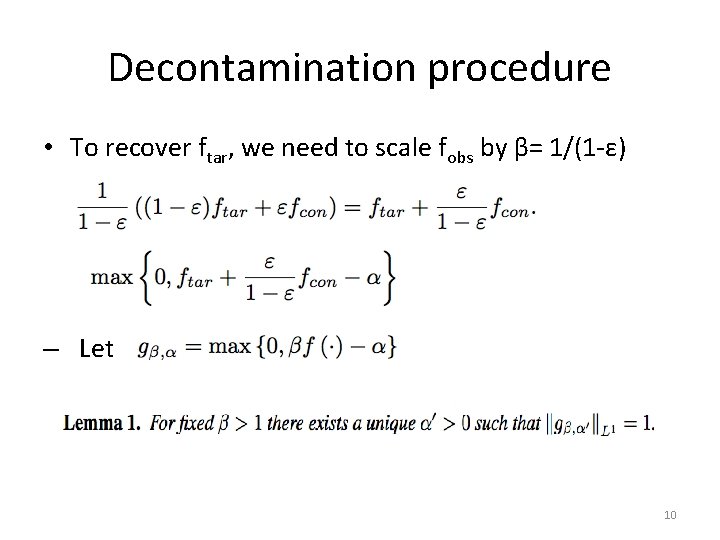
Decontamination procedure • To recover ftar, we need to scale fobs by β= 1/(1 -ε) – Let 10

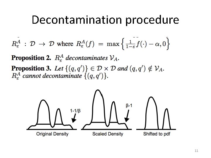
Decontamination procedure 11

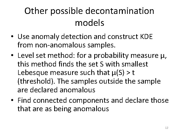
Other possible decontamination models • Use anomaly detection and construct KDE from non-anomalous samples. • Level set method: for a probability measure μ, this method finds the set S with smallest Lebesque measure such that μ(S) > t (threshold). The samples outside the sample are declared anomalous • Find connected components and declare those that are as being anomalous 12

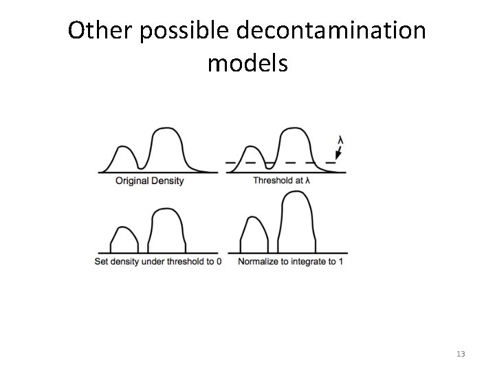
Other possible decontamination models 13

Scaled Projection Kernel Density Estimator • Let’s consider approximating Raε in a finite sample situation. Let f in L 2(R 2) be a pdf and X 1, …, Xn be samples from f. Let kσ(x, x’) be a smoothing kernel with bandwidth σ. • The classic density estimator is: • Since we do not know ε, we will scale β > 1 14

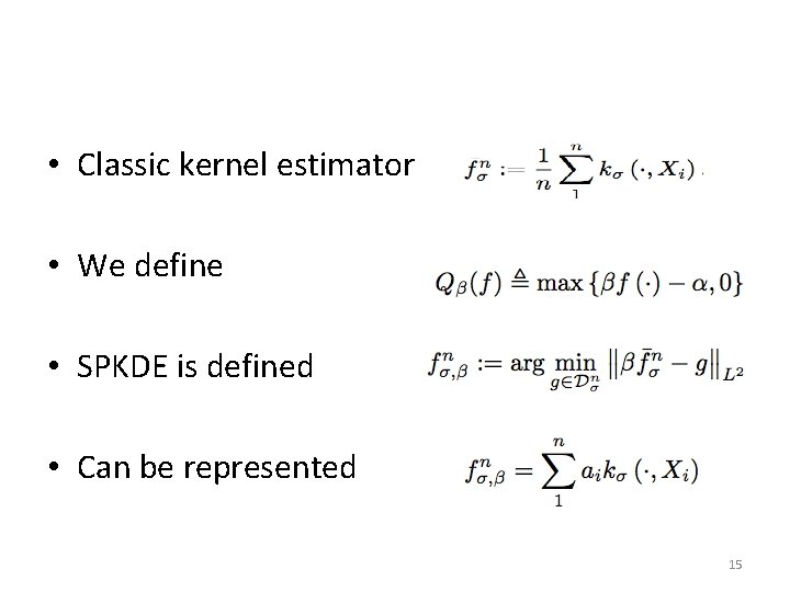
• Classic kernel estimator • We define • SPKDE is defined • Can be represented 15

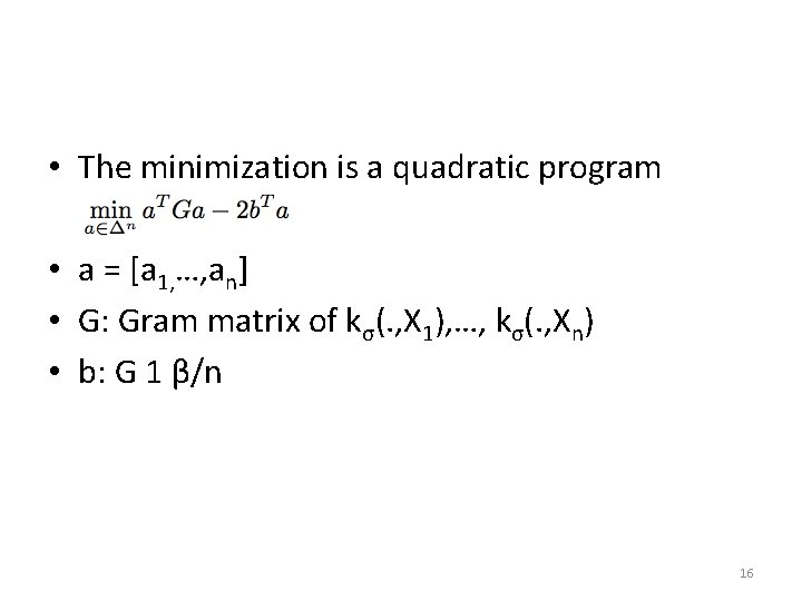
• The minimization is a quadratic program • a = [a 1, …, an] • G: Gram matrix of kσ(. , X 1), …, kσ(. , Xn) • b: G 1 β/n 16

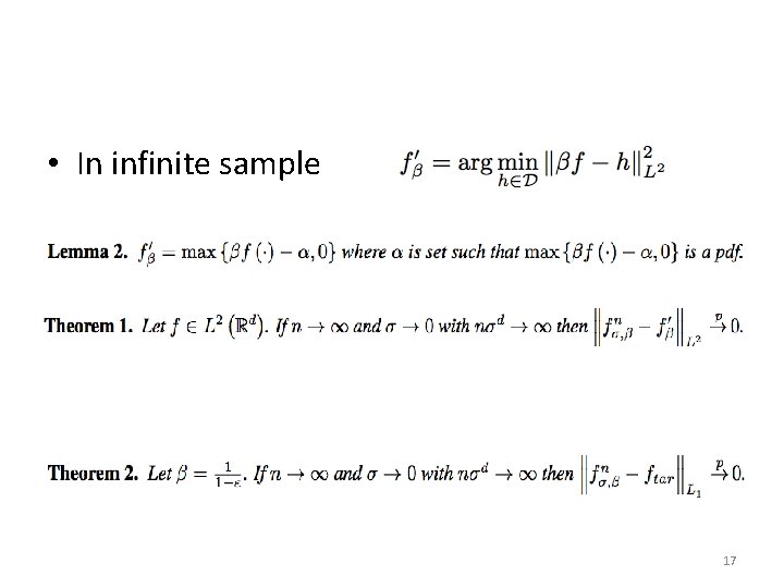
• In infinite sample SKPDE decontamination 17

Experiment and conclusion Datasets • To show SPKDE properties: – Used Synthetic data – Idealized experiment where contamination is uniform – Sample size of 500 and ε = 0. 2 therefore β = 1. 25 • For the remaining experiments: – 12 classification datasets – ε = 0, 0. 05, 0. 1, 0. 25, 0. 3 – Each test is performed on 15 permutations of the dataset 18

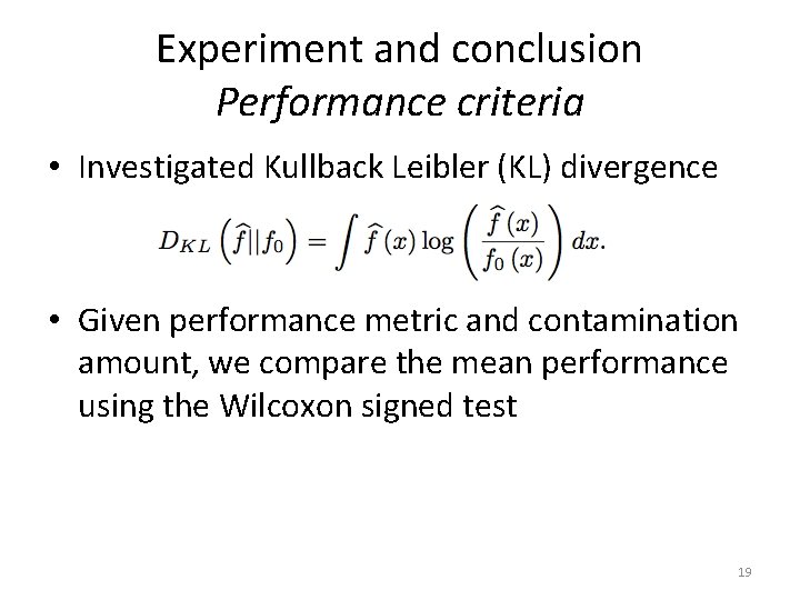
Experiment and conclusion Performance criteria • Investigated Kullback Leibler (KL) divergence • Given performance metric and contamination amount, we compare the mean performance using the Wilcoxon signed test 19

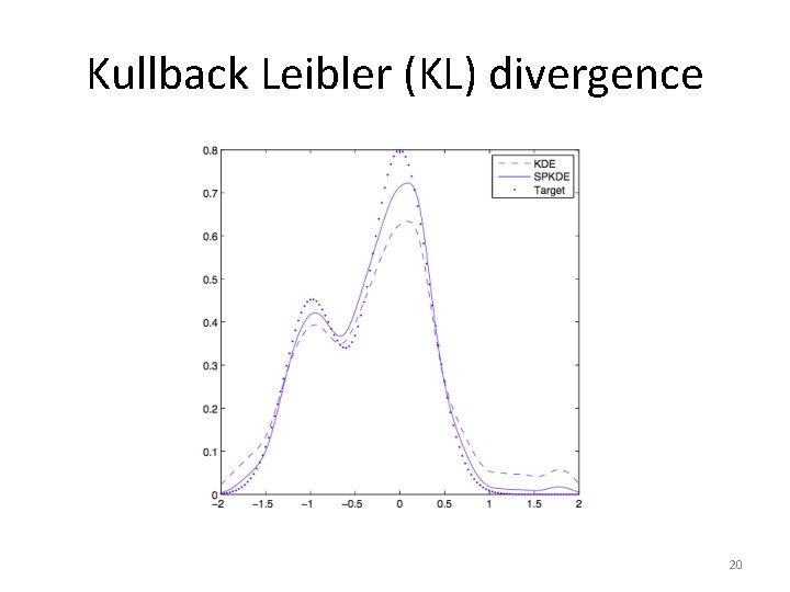
Kullback Leibler (KL) divergence 20

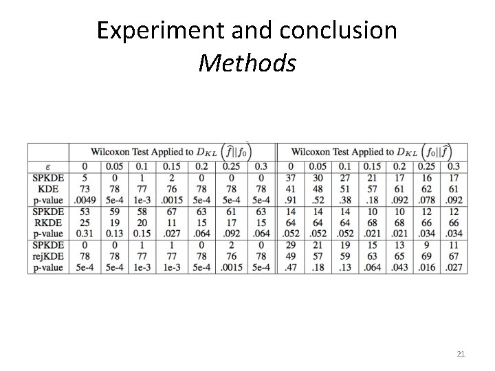
Experiment and conclusion Methods 21

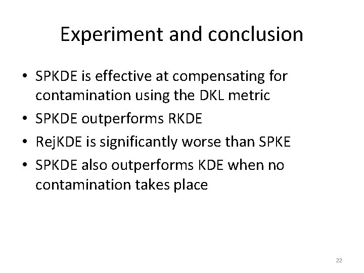
Experiment and conclusion • SPKDE is effective at compensating for contamination using the DKL metric • SPKDE outperforms RKDE • Rej. KDE is significantly worse than SPKE • SPKDE also outperforms KDE when no contamination takes place 22

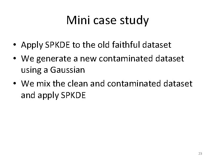
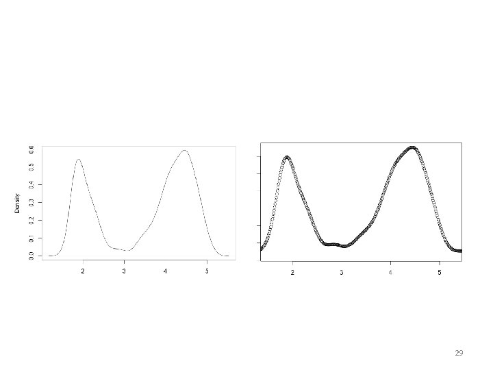
Mini case study • Apply SPKDE to the old faithful dataset • We generate a new contaminated dataset using a Gaussian • We mix the clean and contaminated dataset and apply SPKDE 23

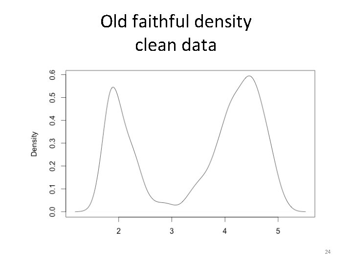
Old faithful density clean data 24

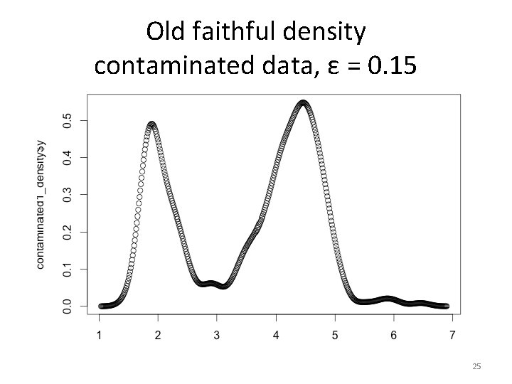
Old faithful density contaminated data, ε = 0. 15 25

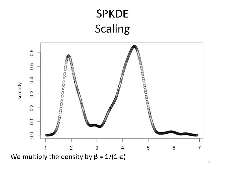
SPKDE Scaling We multiply the density by β = 1/(1 -ε) 26

Shifting • Search for uniform function that has matches highest number of points in distribution • Slice the uniform function from the distribution – Start with threshold and count how many points are close – Increase threshold until number of points decreases – Slice those points from distribution 27

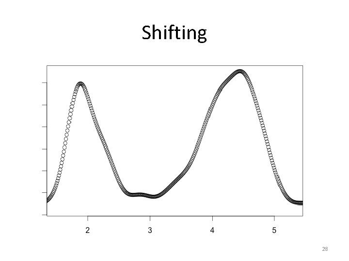
Shifting 28

29

Conclusion • Paper presents a way to construct a robust kernel density estimation • Makes a number of assumptions – Contamination rate is known – The contamination is uniform (Shape of distribution does not change) • You need more information about the contamination – Distribution and contamination rate 30