Robotic Mapping A Survey Sebastian Thrun 2002 Presentation

Robotic Mapping: A Survey Sebastian Thrun, 2002 Presentation by David Black-Schaffer and Kristof Richmond

Historical Overview n Metric Mapping n n Geometric representations Occupancy Grids Larger maps much more computationally intensive Topological Mapping n n n Milestones with connections Require navigation information Hard to scale

The Problems n Measurement noise n n Map size n n High resolution maps can be very large Correspondence n n Sensor and Position noise is not independent Do multiple measurements at different times correspond to the same object? Dynamic environments n Most current algorithms assume a static environment

Current State of Mapping n Algorithms n n n Robust for static, structured, and limited-size environments Probabilistic Correspondence Problem Incremental vs. Multi-pass Unsolved Areas n n Dynamic environments Planning exploration paths of unknown environments

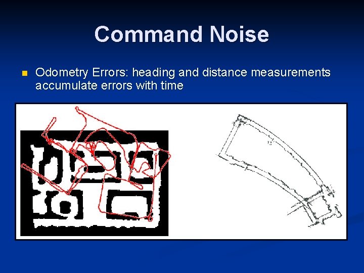
Command Noise n Odometry Errors: heading and distance measurements accumulate errors with time

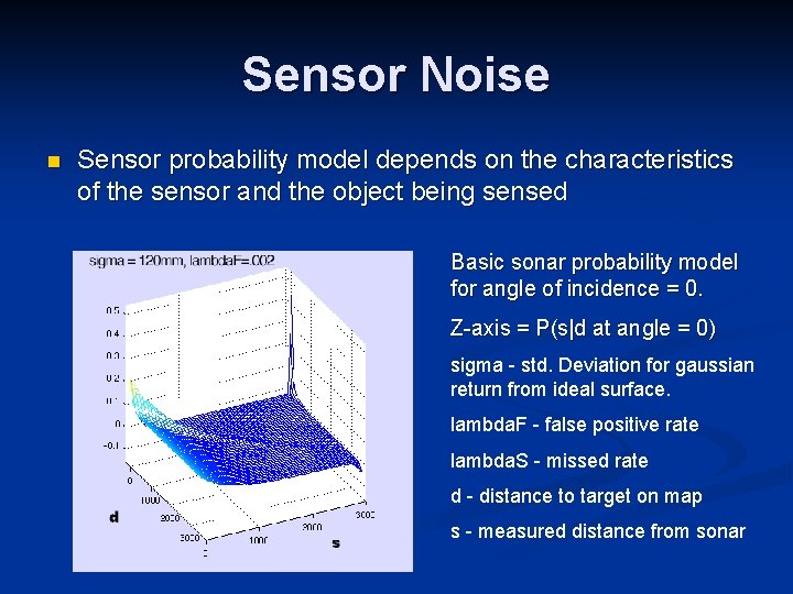
Sensor Noise n Sensor probability model depends on the characteristics of the sensor and the object being sensed Basic sonar probability model for angle of incidence = 0. Z-axis = P(s|d at angle = 0) sigma - std. Deviation for gaussian return from ideal surface. lambda. F - false positive rate lambda. S - missed rate d - distance to target on map s - measured distance from sonar

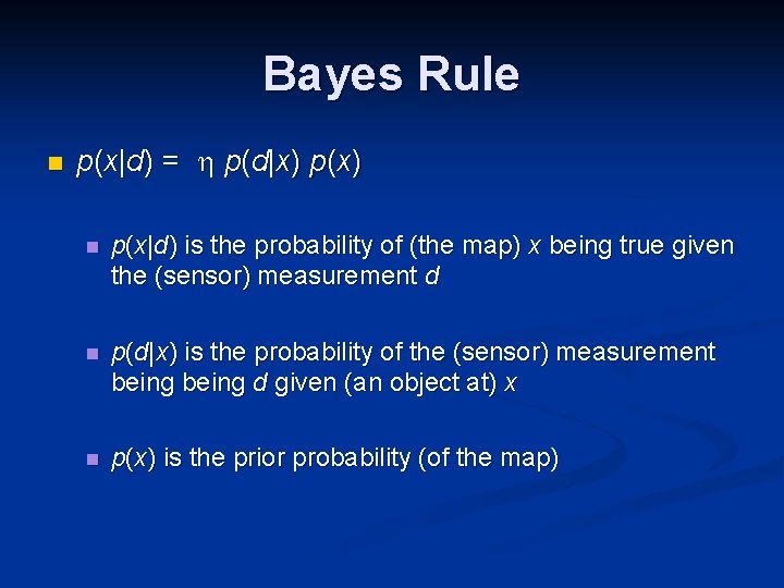
Bayes Rule n p(x|d) = p(d|x) p(x) n p(x|d) is the probability of (the map) x being true given the (sensor) measurement d n p(d|x) is the probability of the (sensor) measurement being d given (an object at) x n p(x) is the prior probability (of the map)

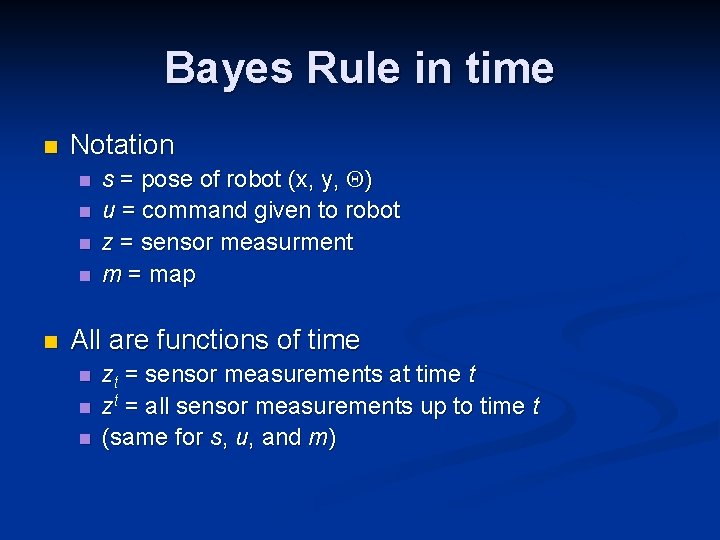
Bayes Rule in time n Notation n n s = pose of robot (x, y, ) u = command given to robot z = sensor measurment m = map All are functions of time n n n zt = sensor measurements at time t zt = all sensor measurements up to time t (same for s, u, and m)

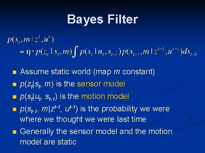
Bayes Filter n Assume static world (map m constant) n p(zt|st, m) is the sensor model n p(st|ut, st-1) is the motion model n p(st-1, m|zt-1, ut-1) is the probability we were where we thought we were last time n Generally the sensor model and the motion model are static

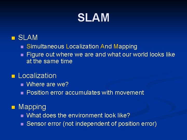
SLAM n n n Localization n Simultaneous Localization And Mapping Figure out where we are and what our world looks like at the same time Where are we? Position error accumulates with movement Mapping n n What does the environment look like? Sensor error (not independent of position error)

SLAM Example Thrun, Sebastian. “Animation of On-line mapping with Monte Carlo Localization”

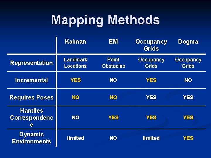
Mapping Methods Kalman EM Occupancy Grids Dogma Representation Landmark Locations Point Obstacles Occupancy Grids Incremental YES NO Requires Poses NO NO YES Handles Correspondenc e NO YES YES Dynamic Environments limited NO limited YES

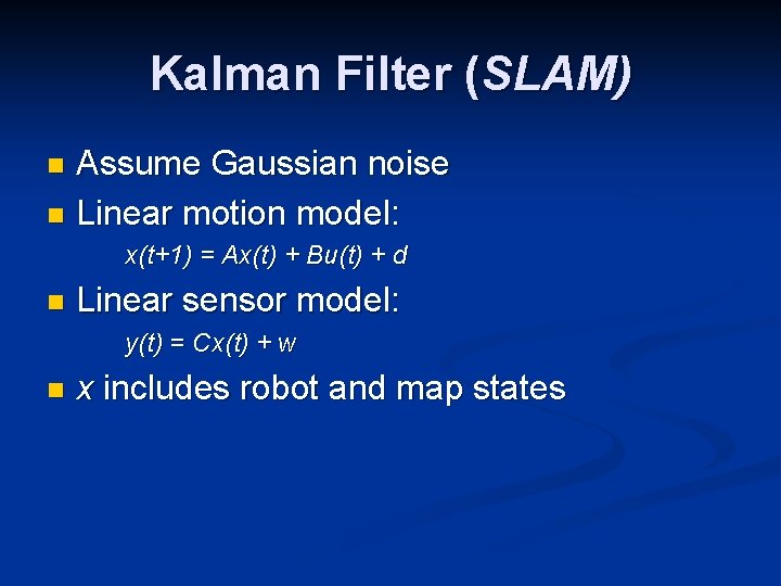
Kalman Filter (SLAM) Assume Gaussian noise n Linear motion model: n x(t+1) = Ax(t) + Bu(t) + d n Linear sensor model: y(t) = Cx(t) + w n x includes robot and map states

Kalman Filter Performance n Pros: n n Cons: n n Full (Gaussian) posterior probabilities Incremental Good convergence Limited model Correspondence problem Limited map size Improvements: Lu/Milios n n Improves correspondence Non-incremental

Newman, Paul. “Navigating in a Building Site - Closed Loop CML”

Expectation Maximization (EM) Find most likely map (and poses) n Expectation step (E-step) n n n Maximization step (M-step) n n Calculate probabilities of robot poses for current guess of map Calculate single most likely map for distribution of robot poses Iterate

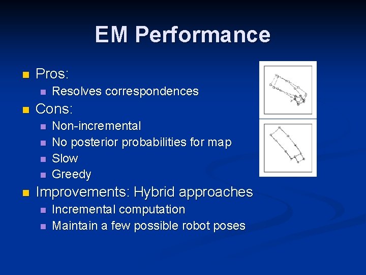
EM Performance n Pros: n n Cons: n n n Resolves correspondences Non-incremental No posterior probabilities for map Slow Greedy Improvements: Hybrid approaches n n Incremental computation Maintain a few possible robot poses

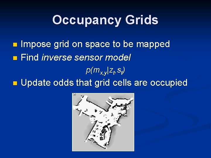
Occupancy Grids Impose grid on space to be mapped n Find inverse sensor model n p(mx, y|zt, st) n Update odds that grid cells are occupied

Occupancy Grid Example Moravec, Hans. “Robust Navigation by Probabilistic Volumetric Sensing’’

Occupancy Grids n Pros n n n Simple Accurate Incremental Cons n n Require known poses Independence assumptions Extensions: Object Maps n Reduced memory requirements n Better for dynamic environments n Limited by available object models

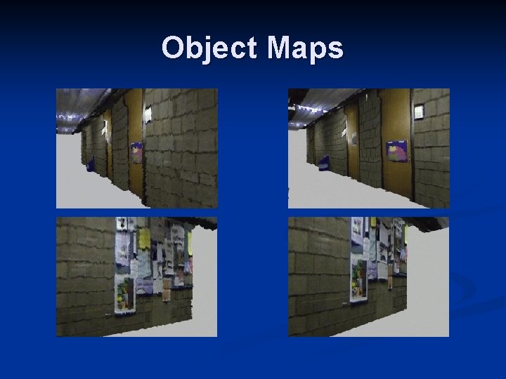
Object Maps

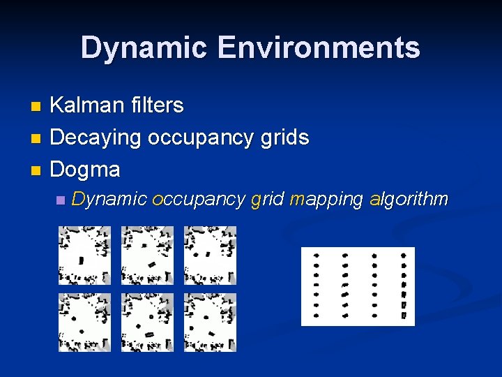
Dynamic Environments Kalman filters n Decaying occupancy grids n Dogma n n Dynamic occupancy grid mapping algorithm