Robot Homing Workshop 1 The Camera Prospective Projection

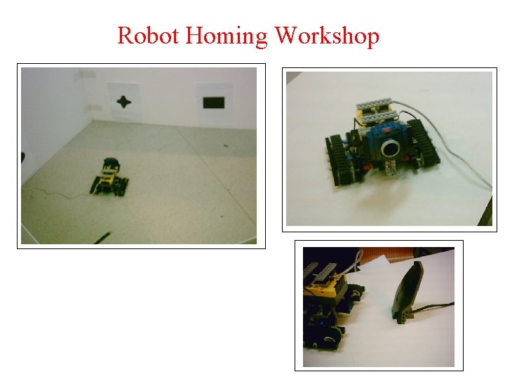
Robot Homing Workshop

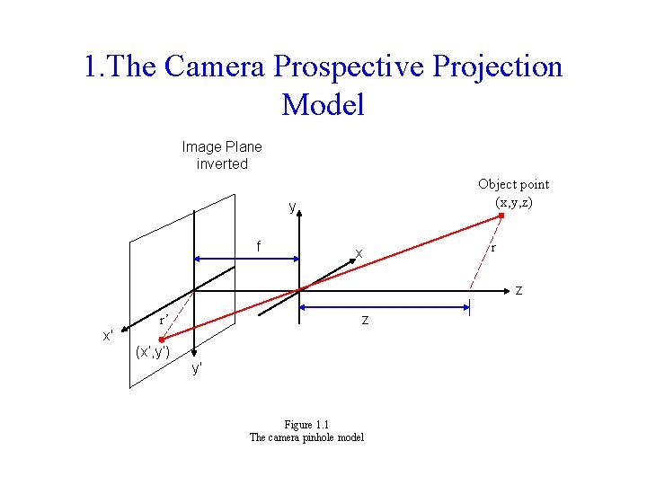
1. The Camera Prospective Projection Model Image Plane inverted Object point (x, y, z) y f x r z z r’ x' (x’, y’) y' Figure 1. 1 The camera pinhole model

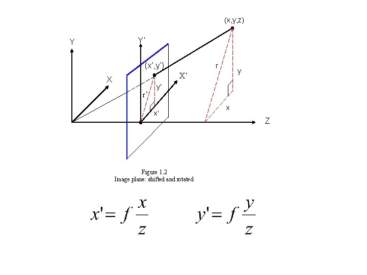
(x, y, z) Y’ Y (x’, y’) r y X’ X r’ y’ x’ Figure 1. 2 Image plane: shifted and rotated x Z

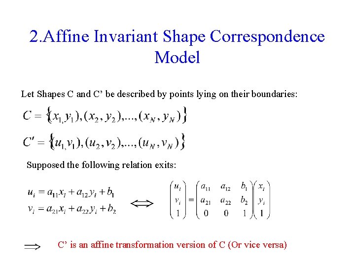
2. Affine Invariant Shape Correspondence Model Let Shapes C and C’ be described by points lying on their boundaries: Supposed the following relation exits: C’ is an affine transformation version of C (Or vice versa)

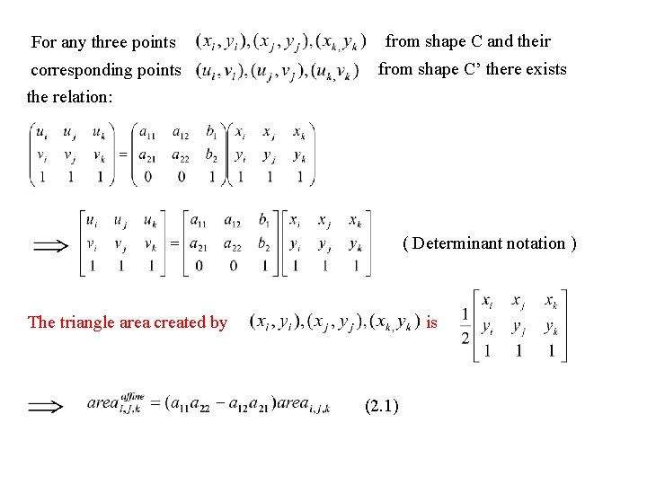
For any three points from shape C and their corresponding points the relation: from shape C’ there exists ( Determinant notation ) is The triangle area created by (2. 1)

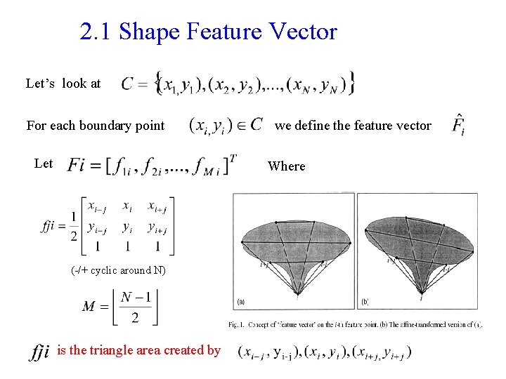
2. 1 Shape Feature Vector Let’s look at For each boundary point Let we define the feature vector Where (-/+ cyclic around N) is the triangle area created by

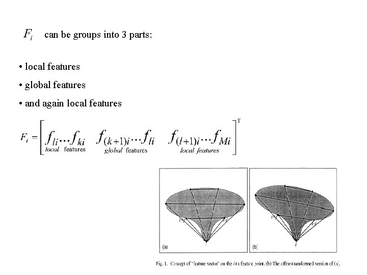
can be groups into 3 parts: • local features • global features • and again local features

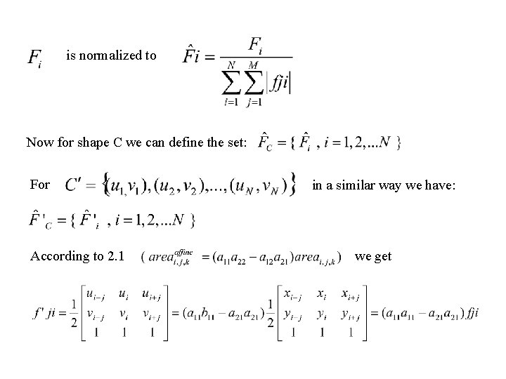
is normalized to Now for shape C we can define the set: For According to 2. 1 in a similar way we have: we get

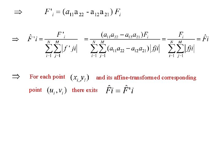
For each point and its affine-transformed corresponding there exits

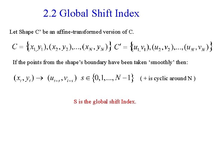
2. 2 Global Shift Index Let Shape C’ be an affine-transformed version of C. If the points from the shape’s boundary have been taken ‘smoothly’ then: ( + is cyclic around N ) S is the global shift Index.

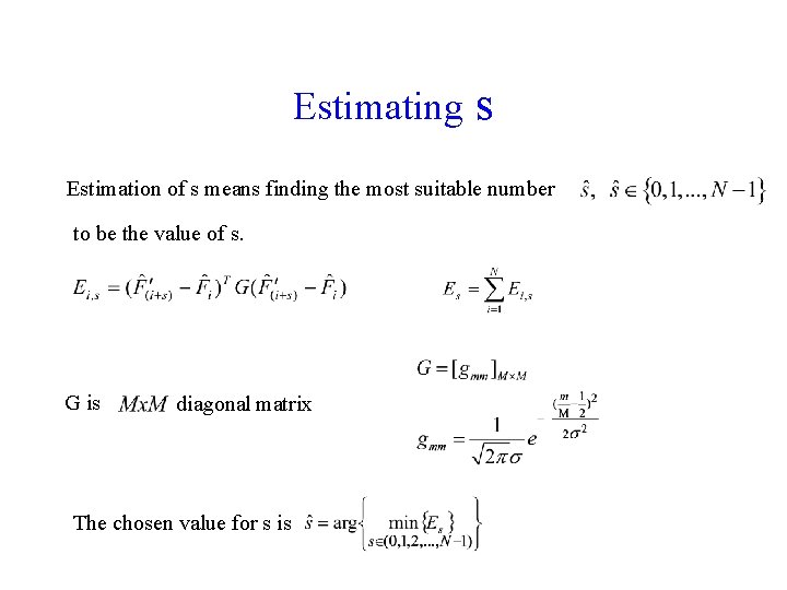
Estimating s Estimation of s means finding the most suitable number to be the value of s. G is diagonal matrix The chosen value for s is

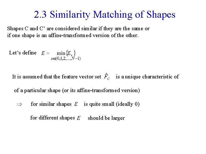
2. 3 Similarity Matching of Shapes C and C’ are considered similar if they are the same or if one shape is an affine-transformed version of the other. Let’s define It is assumed that the feature vector set is a unique characteristic of of a particular shape (or its affine-transformed version) for similar shapes for different shapes is quite small (ideally 0) should be larger

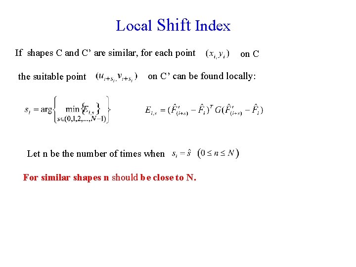
Local Shift Index If shapes C and C’ are similar, for each point the suitable point on C’ can be found locally: Let n be the number of times when For similar shapes n should be close to N.

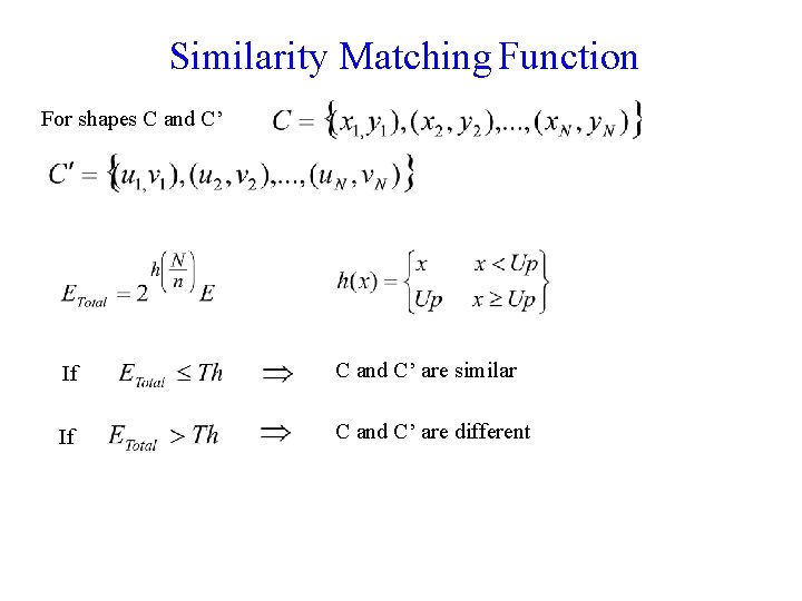
Similarity Matching Function For shapes C and C’ If C and C’ are similar If C and C’ are different

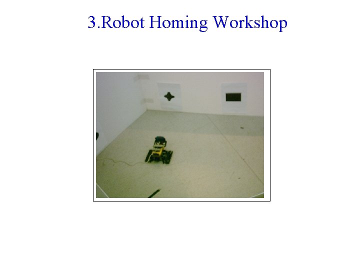
3. Robot Homing Workshop

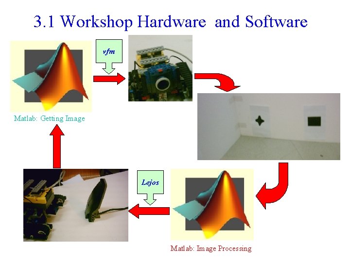
3. 1 Workshop Hardware and Software vfm Matlab: Getting Image Lejos Matlab: Image Processing

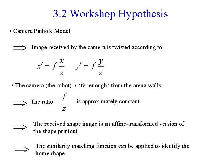
3. 2 Workshop Hypothesis • Camera Pinhole Model Image received by the camera is twisted according to: • The camera (the robot) is ‘far enough’ from the arena walls The ratio is approximately constant The received shape image is an affine-transformed version of the shape printout. The similarity matching function can be applied to identify the home shape.

3. 3 The Matlab Program Aspects • Traveling around the arena and grabbing the wall images • Analyzing the received images and retrieving the shape figures • Determine whether the retrieved shape is the home shape • Traveling towards the home shape when it has been detected

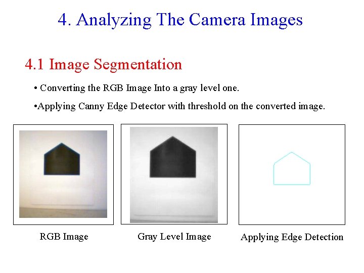
4. Analyzing The Camera Images 4. 1 Image Segmentation • Converting the RGB Image Into a gray level one. • Applying Canny Edge Detector with threshold on the converted image. RGB Image Gray Level Image Applying Edge Detection

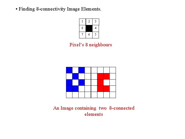
• Finding 8 -connectivity Image Elements. 1 2 8 7 3 4 6 5 Pixel’s 8 neighbours An Image containing two 8 -connected elements

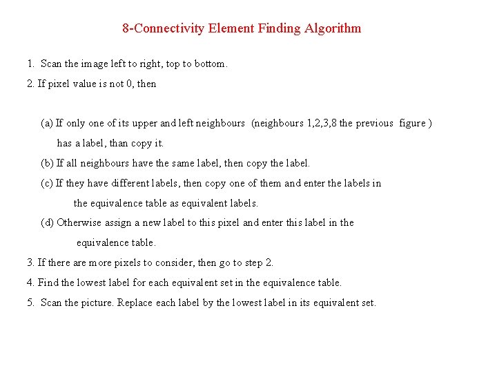
8 -Connectivity Element Finding Algorithm 1. Scan the image left to right, top to bottom. 2. If pixel value is not 0, then (a) If only one of its upper and left neighbours (neighbours 1, 2, 3, 8 the previous figure ) has a label, than copy it. (b) If all neighbours have the same label, then copy the label. (c) If they have different labels, then copy one of them and enter the labels in the equivalence table as equivalent labels. (d) Otherwise assign a new label to this pixel and enter this label in the equivalence table. 3. If there are more pixels to consider, then go to step 2. 4. Find the lowest label for each equivalent set in the equivalence table. 5. Scan the picture. Replace each label by the lowest label in its equivalent set.

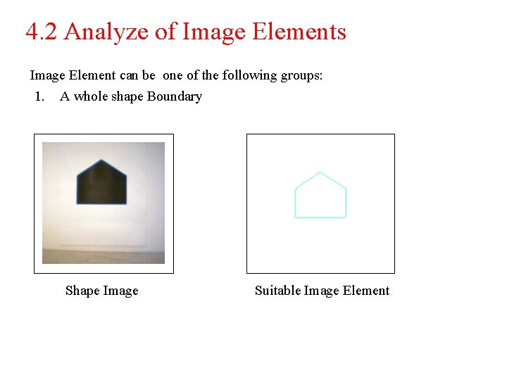
4. 2 Analyze of Image Elements Image Element can be one of the following groups: 1. A whole shape Boundary Shape Image Suitable Image Element

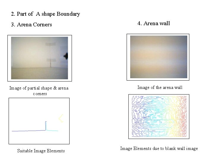
2. Part of A shape Boundary 3. Arena Corners Image of partial shape & arena corners Suitable Image Elements 4. Arena wall Image of the arena wall Image Elements due to blank wall image

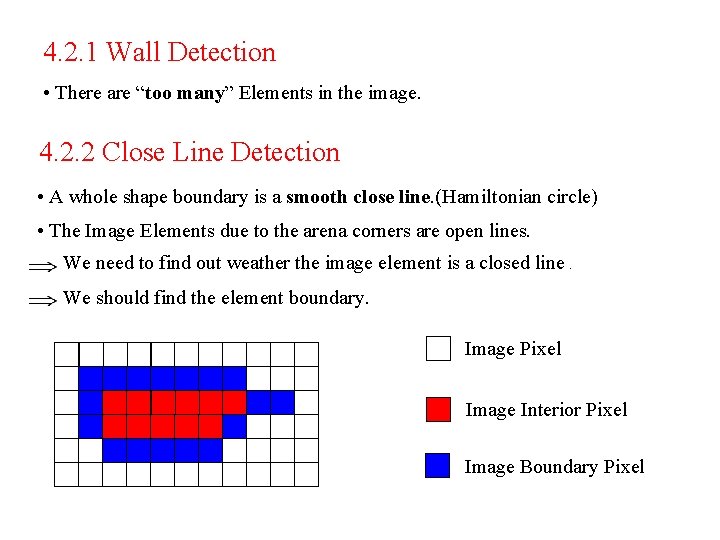
4. 2. 1 Wall Detection • There are “too many” Elements in the image. 4. 2. 2 Close Line Detection • A whole shape boundary is a smooth close line. (Hamiltonian circle) • The Image Elements due to the arena corners are open lines. We need to find out weather the image element is a closed line. We should find the element boundary. Image Pixel Image Interior Pixel Image Boundary Pixel

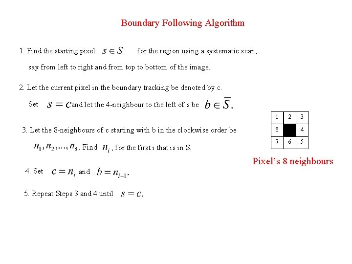
Boundary Following Algorithm 1. Find the starting pixel for the region using a systematic scan, say from left to right and from top to bottom of the image. 2. Let the current pixel in the boundary tracking be denoted by c. Set and let the 4 -neighbour to the left of s be 1 3. Let the 8 -neighbours of c starting with b in the clockwise order be. Find , for the first i that is in S. 2 8 7 3 4 6 5 Pixel’s 8 neighbours 4. Set and 5. Repeat Steps 3 and 4 until

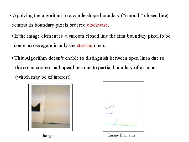
• Applying the algorithm to a whole shape boundary (“smooth” closed line) returns its boundary pixels ordered clockwise. • If the image element is a smooth closed line the first boundary pixel to be come across again is only the starting one c. • This Algorithm doesn’t enable to distinguish between open lines due to the arena corners and open lines due to partial boundary of a shape (which may be of interest). Image Elements

4. 2. 3 Detection of the Home Shape • The boundary of the shape considered home is a closed line. • The (synthetic) home figure is stored in the robot data base. (simply a file) and its boundary is of course closed. We can use the matching algorithm described above. • Sampling in “smooth manner” N points from the home boundary as in the data base. • Sampling in “smooth manner” N point from the received shape boundary (suitable element pixels) • Applying the matching algorithm

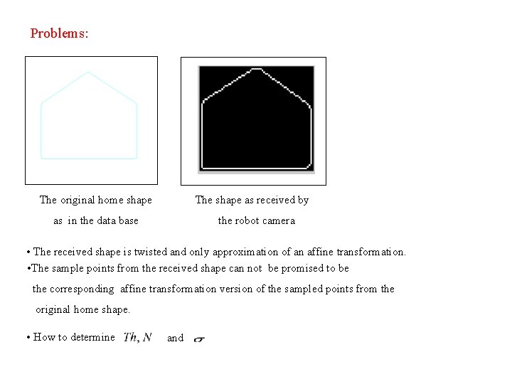
Problems: The original home shape The shape as received by as in the data base the robot camera • The received shape is twisted and only approximation of an affine transformation. • The sample points from the received shape can not be promised to be the corresponding affine transformation version of the sampled points from the original home shape. • How to determine and

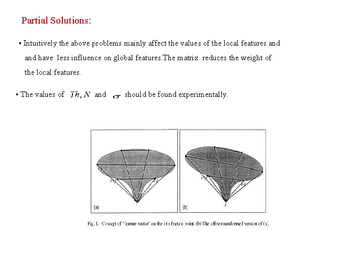
Partial Solutions: • Intuitively the above problems mainly affect the values of the local features and have less influence on global features. The matrix reduces the weight of the local features. • The values of and should be found experimentally.

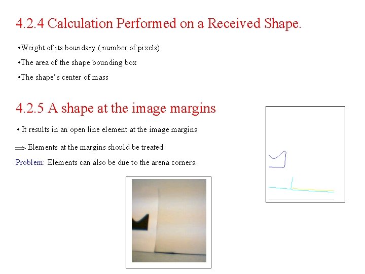
4. 2. 4 Calculation Performed on a Received Shape. • Weight of its boundary ( number of pixels) • The area of the shape bounding box • The shape’s center of mass 4. 2. 5 A shape at the image margins • It results in an open line element at the image margins Elements at the margins should be treated. Problem: Elements can also be due to the arena corners.

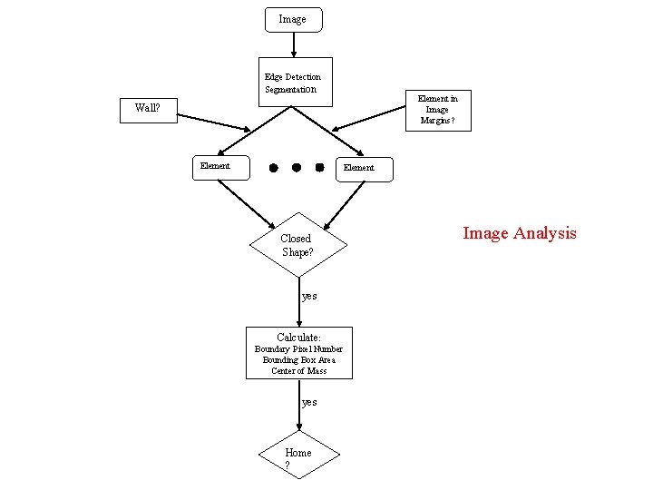
Image Edge Detection Segmentation Element in Image Margins? Wall? Element Closed Shape? yes Calculate : Boundary Pixel Number Bounding Box Area Center of Mass yes Home ? Image Analysis

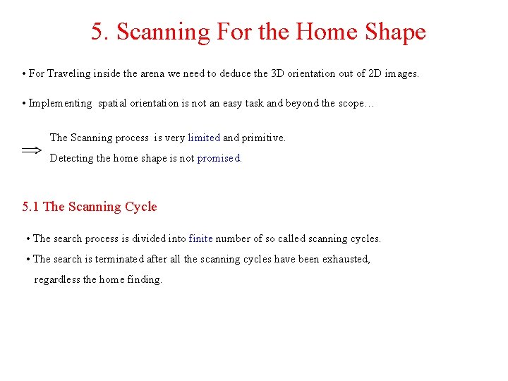
5. Scanning For the Home Shape • For Traveling inside the arena we need to deduce the 3 D orientation out of 2 D images. • Implementing spatial orientation is not an easy task and beyond the scope… The Scanning process is very limited and primitive. Detecting the home shape is not promised. 5. 1 The Scanning Cycle • The search process is divided into finite number of so called scanning cycles. • The search is terminated after all the scanning cycles have been exhausted, regardless the home finding.

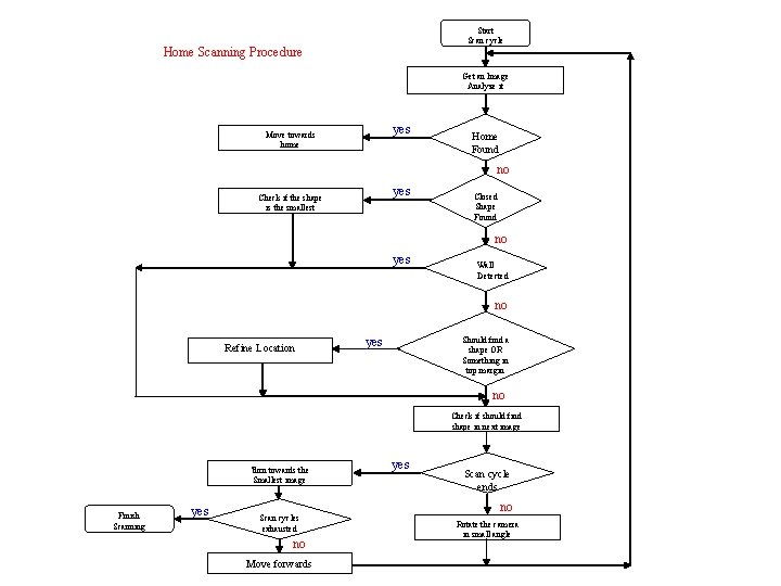
Start Scan cycle Home Scanning Procedure Get an Image Analyze it yes Move towards home Home Found no yes Check if the shape is the smallest Closed Shape Found no yes Wall Detected no Refine Location yes Should find a shape OR Something in top margin no Check if should find shape in next image Turn towards the Smallest image Finish Scanning yes Scan cycles exhausted no Move forwards yes Scan cycle ends no Rotate the camera in small angle

5. 2 The Refine Location Procedure. The procedure handles two case: • There is an element at the top margin of the image so it might be a part of a shape to which the robot camera is to close. • The current image analysis yields no close shape whereas according to the previous image a shape should have been found. (element at the left/right margin) Problem: Because of the insufficient segmentation the elements can be due to the arena walls, texture and etc. A finite number of trials should be taken in order to find a shape.

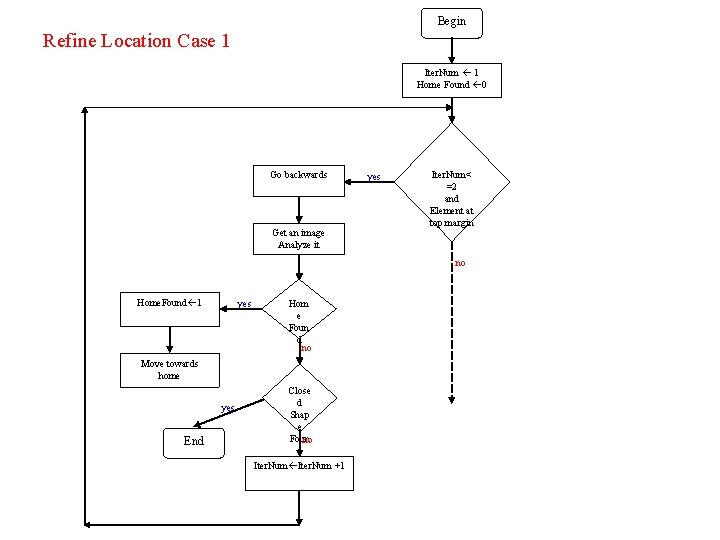
Begin Refine Location Case 1 Iter. Num 1 Home Found 0 Go backwards Get an image Analyze it yes Iter. Num< =2 and Element at top margin no Home. Found 1 yes Hom e Foun d no Move towards home yes End Close d Shap e Foun no d Iter. Num +1

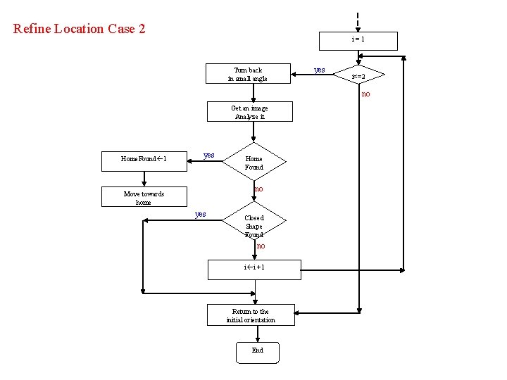
Refine Location Case 2 i=1 Turn back in small angle yes i<=2 no Get an image Analyze it Home. Found 1 yes Home Found no Move towards home yes Closed Shape Found no i i +1 Return to the initial orientation End

5. 3 Moving towards Home Procedure • Once the home shape has been detected, the robot moved towards it. Problem: The home shape doesn’t have to be in the image center so while moving towards it the shape might be out of the sight field of the camera. • Calculating the home shape center of mass. • The robot moves forward in small “steps” checking after each step if the home shape is still in camera field of sight. • If not, The robot moves backwards to its previous location and turns a “little” towards the home shape according to the location of the shape’s center of mass. Problem: The robot shouldn’t approach the home shape too much, otherwise the affine transformation approximation won’t be correct to be used and the matching algorithm won’t be consistent. • Calculation the area of the home shape bounding box. • If the area is “too large” the robot stops and doesn’t try to get closer.

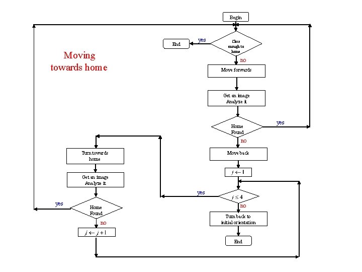
Begin End yes Moving towards home Close enough to home no Move forwards Get an image Analyze it Home Found no Move back Turn towards home Get an image Analyze it yes Home Found no no Turn back to initial orientation End yes