ROAD MAP Terminology The graphical approach Three types

ROAD MAP § Terminology § The graphical approach § Three types of LPs § Simple LP formulations § Compact LP formulations Linear Programming 2021/9/9 1

INTRODUCTION § It is important to learn how to model a practical situation as an LP. § Once you do so, you have “solved” the problem. § This process is typically called LP formulation or modeling. § Here we will give you two examples of LP formulation. § Then we formulate large-scale problems with compact formulations. Linear Programming 2021/9/9 2

A PRODUCT MIX PROBLEM § We produce several products to sell. § Each product requires some resources. Resources are limited. § We want to maximize the total sales revenue with available resources. Linear Programming 2021/9/9 3

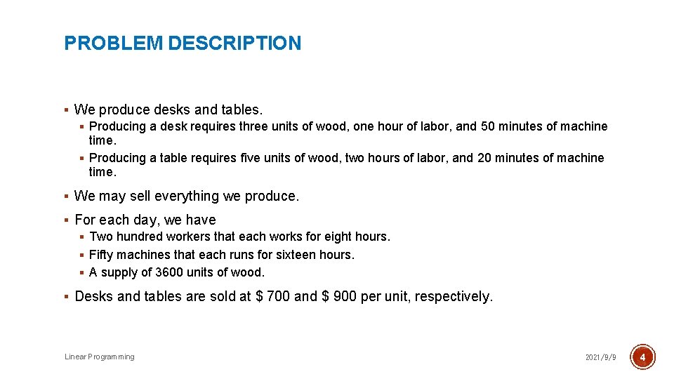
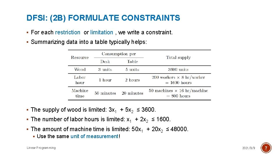
PROBLEM DESCRIPTION § We produce desks and tables. § Producing a desk requires three units of wood, one hour of labor, and 50 minutes of machine time. § Producing a table requires five units of wood, two hours of labor, and 20 minutes of machine time. § We may sell everything we produce. § For each day, we have § Two hundred workers that each works for eight hours. § Fifty machines that each runs for sixteen hours. § A supply of 3600 units of wood. § Desks and tables are sold at $ 700 and $ 900 per unit, respectively. Linear Programming 2021/9/9 4

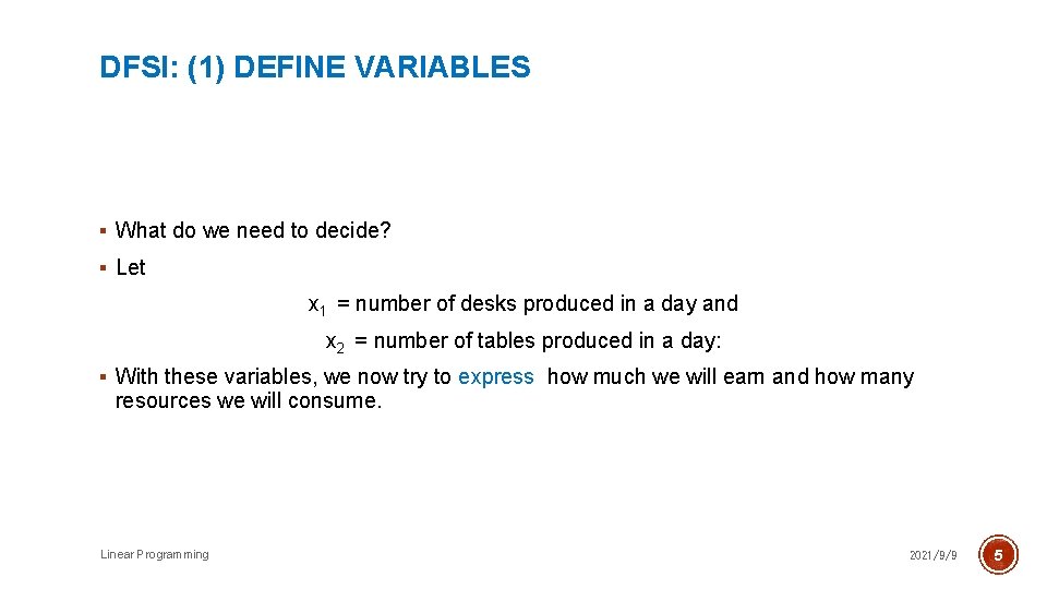
DFSI: (1) DEFINE VARIABLES § What do we need to decide? § Let x 1 = number of desks produced in a day and x 2 = number of tables produced in a day: § With these variables, we now try to express how much we will earn and how many resources we will consume. Linear Programming 2021/9/9 5

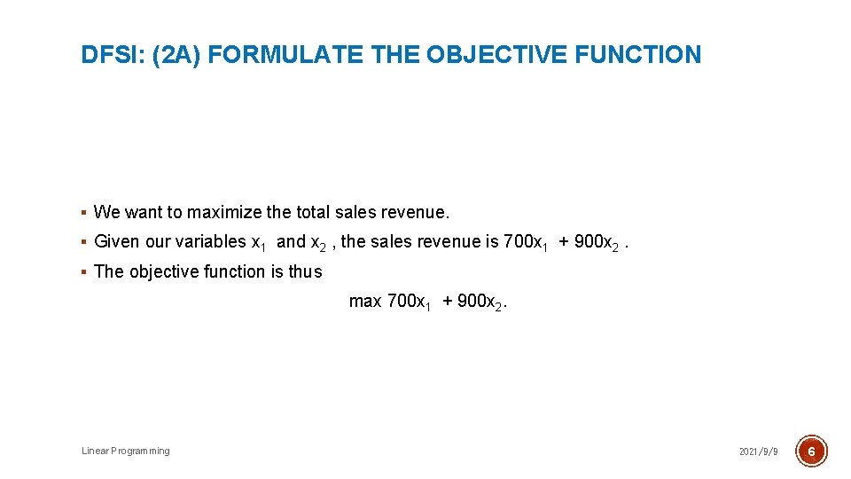
DFSI: (2 A) FORMULATE THE OBJECTIVE FUNCTION § We want to maximize the total sales revenue. § Given our variables x 1 and x 2 , the sales revenue is 700 x 1 + 900 x 2. § The objective function is thus max 700 x 1 + 900 x 2. Linear Programming 2021/9/9 6

DFSI: (2 B) FORMULATE CONSTRAINTS § For each restriction or limitation , we write a constraint. § Summarizing data into a table typically helps: § The supply of wood is limited: 3 x 1 + 5 x 2 ≤ 3600. § The number of labor hours is limited: x 1 + 2 x 2 ≤ 1600. § The amount of machine time is limited: 50 x 1 + 20 x 2 ≤ 48000. § Use the same unit of measurement! Linear Programming 2021/9/9 7

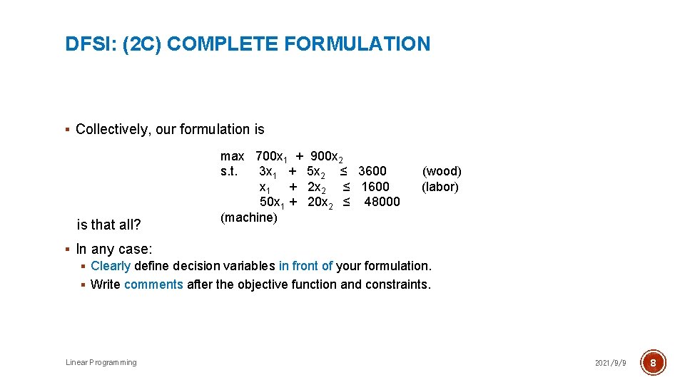
DFSI: (2 C) COMPLETE FORMULATION § Collectively, our formulation is is that all? max 700 x 1 + 900 x 2 s. t. 3 x 1 + 5 x 2 ≤ 3600 x 1 + 2 x 2 ≤ 1600 50 x 1 + 20 x 2 ≤ 48000 (machine) (wood) (labor) § In any case: § Clearly define decision variables in front of your formulation. § Write comments after the objective function and constraints. Linear Programming 2021/9/9 8

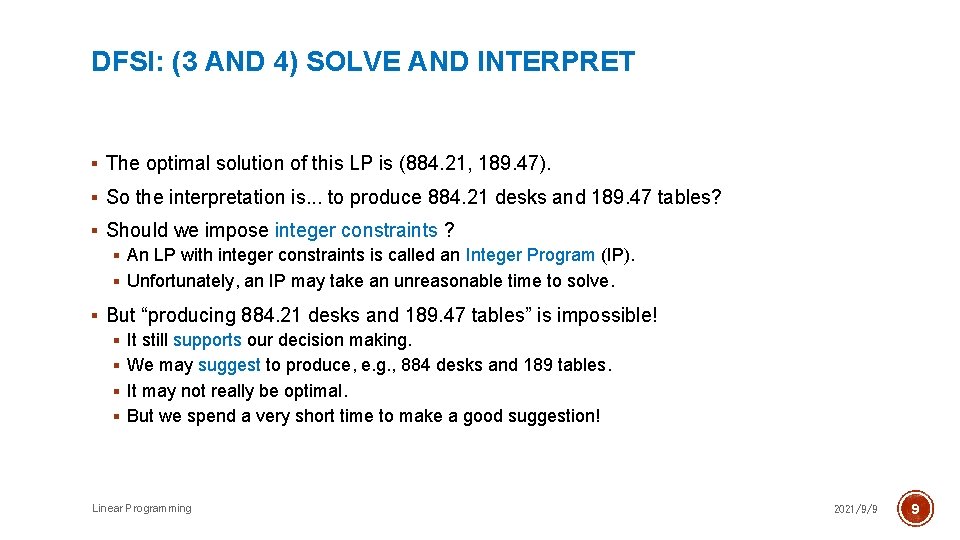
DFSI: (3 AND 4) SOLVE AND INTERPRET § The optimal solution of this LP is (884. 21, 189. 47). § So the interpretation is. . . to produce 884. 21 desks and 189. 47 tables? § Should we impose integer constraints ? § An LP with integer constraints is called an Integer Program (IP). § Unfortunately, an IP may take an unreasonable time to solve. § But “producing 884. 21 desks and 189. 47 tables” is impossible! § It still supports our decision making. § We may suggest to produce, e. g. , 884 desks and 189 tables. § It may not really be optimal. § But we spend a very short time to make a good suggestion! Linear Programming 2021/9/9 9

PRODUCE AND STORE! § When we are making decisions, we may also consider what will happen in the future. § This creates multi-period problems. § In many cases, products produced today may be stored and then sold in the future. § Maybe daily capacity is not enough. § Maybe production is cheaper today. § Maybe the price is higher in the future. § So the production decision must be jointly considered with the inventory decision. Linear Programming 2021/9/9 10

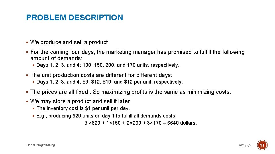
PROBLEM DESCRIPTION § We produce and sell a product. § For the coming four days, the marketing manager has promised to fulfill the following amount of demands: § Days 1, 2, 3, and 4: 100, 150, 200, and 170 units, respectively. § The unit production costs are different for different days: § Days 1, 2, 3, and 4: $9, $12, $10, and $12 per unit, respectively. § The prices are all fixed. So maximizing profits is the same as minimizing costs. § We may store a product and sell it later. § The inventory cost is $1 per unit per day. § E. g. , producing 620 units on day 1 to fulfill all demands costs 9 × 620 + 1× 150 + 2× 200 + 3× 170 = 6640 dollars: Linear Programming 2021/9/9 11

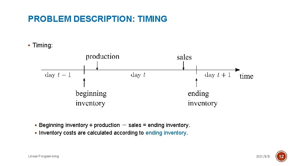
PROBLEM DESCRIPTION: TIMING § Timing: § Beginning inventory + production － sales = ending inventory. § Inventory costs are calculated according to ending inventory. Linear Programming 2021/9/9 12

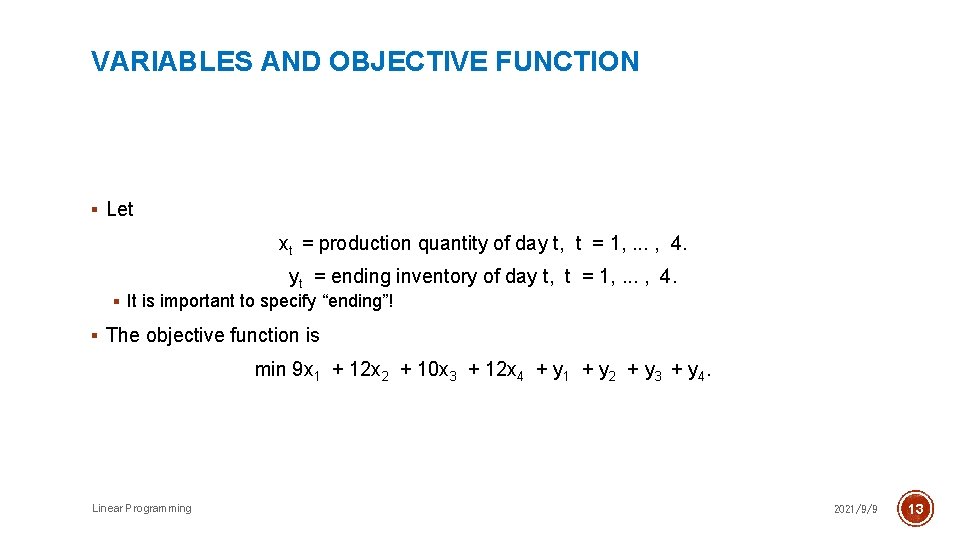
VARIABLES AND OBJECTIVE FUNCTION § Let xt = production quantity of day t, t = 1, . . . , 4. yt = ending inventory of day t, t = 1, . . . , 4. § It is important to specify “ending”! § The objective function is min 9 x 1 + 12 x 2 + 10 x 3 + 12 x 4 + y 1 + y 2 + y 3 + y 4. Linear Programming 2021/9/9 13

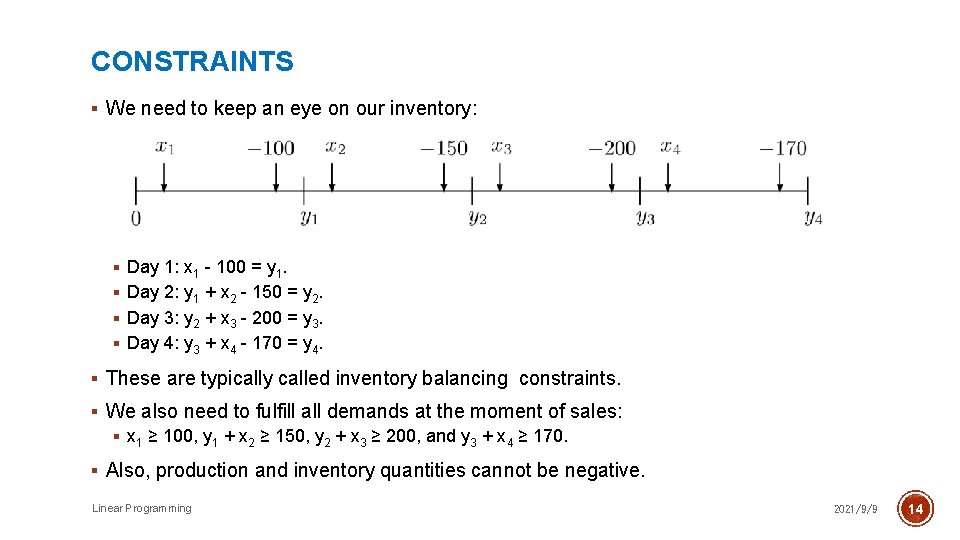
CONSTRAINTS § We need to keep an eye on our inventory: § Day 1: x 1 - 100 = y 1. § Day 2: y 1 + x 2 - 150 = y 2. § Day 3: y 2 + x 3 - 200 = y 3. § Day 4: y 3 + x 4 - 170 = y 4. § These are typically called inventory balancing constraints. § We also need to fulfill all demands at the moment of sales: § x 1 ≥ 100, y 1 + x 2 ≥ 150, y 2 + x 3 ≥ 200, and y 3 + x 4 ≥ 170. § Also, production and inventory quantities cannot be negative. Linear Programming 2021/9/9 14

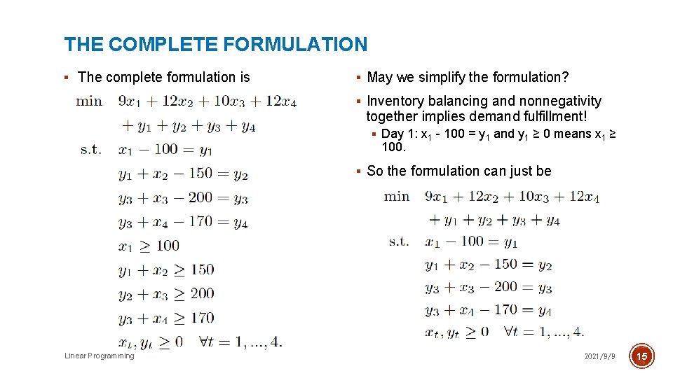
THE COMPLETE FORMULATION § The complete formulation is § May we simplify the formulation? § Inventory balancing and nonnegativity together implies demand fulfillment! § Day 1: x 1 - 100 = y 1 and y 1 ≥ 0 means x 1 ≥ 100. § So the formulation can just be Linear Programming 2021/9/9 15

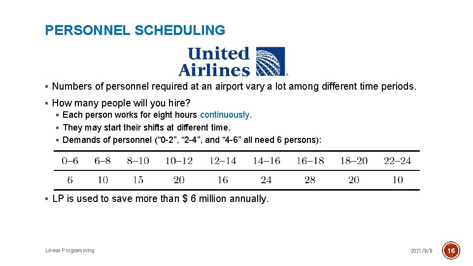
PERSONNEL SCHEDULING § Numbers of personnel required at an airport vary a lot among different time periods. § How many people will you hire? § Each person works for eight hours continuously. § They may start their shifts at different time. § Demands of personnel (“ 0 -2”, “ 2 -4”, and “ 4 -6” all need 6 persons): § LP is used to save more than $ 6 million annually. Linear Programming 2021/9/9 16

ROAD MAP § Terminology § The graphical approach § Three types of LPs § Simple LP formulations § Compact LP formulations Linear Programming 2021/9/9 17

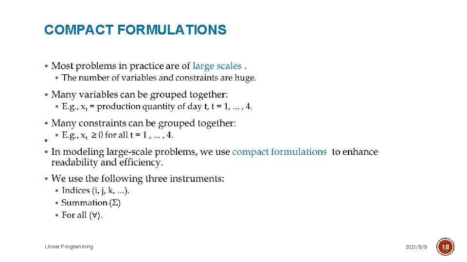
COMPACT FORMULATIONS § Linear Programming 2021/9/9 18

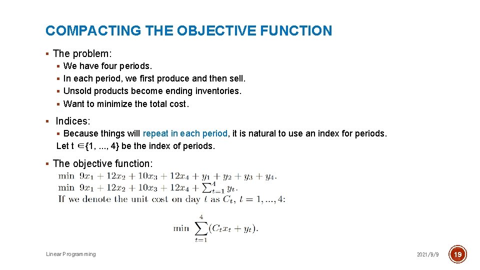
COMPACTING THE OBJECTIVE FUNCTION § The problem: § We have four periods. § In each period, we first produce and then sell. § Unsold products become ending inventories. § Want to minimize the total cost. § Indices: § Because things will repeat in each period, it is natural to use an index for periods. Let t ∈{1, . . . , 4} be the index of periods. § The objective function: Linear Programming 2021/9/9 19

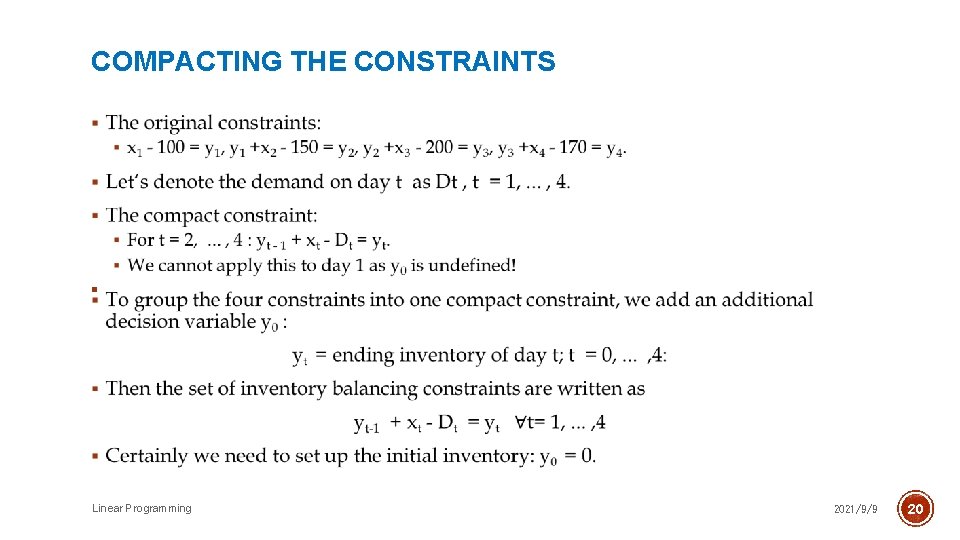
COMPACTING THE CONSTRAINTS § Linear Programming 2021/9/9 20

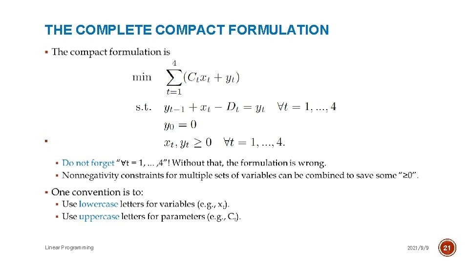
THE COMPLETE COMPACT FORMULATION § Linear Programming 2021/9/9 21

PARAMETER DECLARATION § When creating parameter sets, we write something like denote Ct as the unit production cost on day t, t = 1, . . . , 4: § Do not need to specify values, even though we have those values. § Need to specify the range through indices. § Parameter declarations should be at the beginning of the formulation. § Parameters and variables are just different. § Variables are those to be determined. We do have know there values before we solve the model. § Parameters are given with known values. § Parameters are exogenous and variables are endogenous. Linear Programming 2021/9/9 22