Risk Risk Preferences Insurance Risk and Poverty Consider

Risk, Risk Preferences & Insurance

Risk and Poverty • Consider the following strategies that may help poor households increase their income and leave poverty behind: • • Adopt a new technology Plant a new crop Open a new business Migrate to a city to find a higher paying job • Two key features of these strategies • Require investment (credit markets crucial) • Imply taking risks because payoffs are unknown ex ante What determines if a household is willing and able to make risky investments?

Insights from “Barefoot Hedgefund Managers” • Structure of Employment/Income Generation for the poor in developing countries • • Majority of poor are self-employed Even higher fraction of rural poor are self-employed (on farm and off-farm) Most wage work is casual (day work) Very few households have stable, salaried income earners • Economic risks to self-employed/casual workers are very high • Income risk due to price fluctuations (of output and inputs) • Income risk due to fluctuations in production/output from weather, pests, natural disaster, political change • Additional risks from violence, theft, sickness, death • And access to insurance and other financial instruments to manage risk is limited • Risk and uncertainty make saving, planning and investment both difficult and important • Risk and missing formal/informal risk sharing mechanisms can lead to poverty traps Ex-post: After getting hit by a bad shock, I may not fully recover… Ex-ante: The threat of bad shocks, like a bully, may cause me to choose low return but safer

Expected Utility Framework • In order to understand how people make risky decisions, we need a systematic framework for thinking about the effect of risk on people’s decisions • In other words, we need a framework to characterize peoples’ “risk preferences” • The key idea: Humans are hardwired to favor predictable consumption in the future The Expected Value of an outcome and the Variability of the outcome both matter! How do we represent this preference for both Mean and Variance? • Expected Utility is a convenient way to capture this preference for predictability using simple mathematics • Let’s illustrate by eliciting your OWN risk preferences!

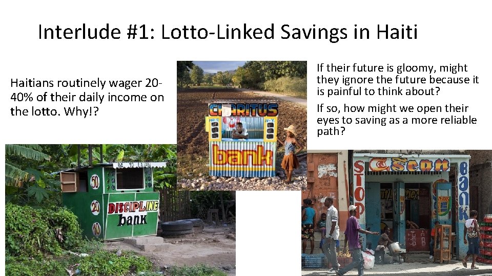
Interlude #1: Lotto-Linked Savings in Haitians routinely wager 2040% of their daily income on the lotto. Why!? If their future is gloomy, might they ignore the future because it is painful to think about? If so, how might we open their eyes to saving as a more reliable path?

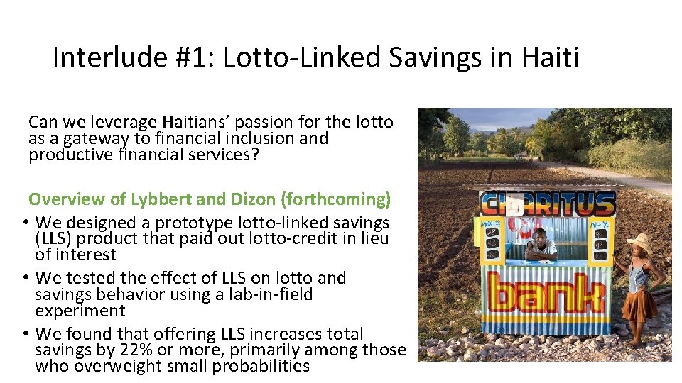
Interlude #1: Lotto-Linked Savings in Haiti Can we leverage Haitians’ passion for the lotto as a gateway to financial inclusion and productive financial services? Overview of Lybbert and Dizon (forthcoming) • We designed a prototype lotto-linked savings (LLS) product that paid out lotto-credit in lieu of interest • We tested the effect of LLS on lotto and savings behavior using a lab-in-field experiment • We found that offering LLS increases total savings by 22% or more, primarily among those who overweight small probabilities

Interlude #2: Experimental Economics • The structure of our Discipline Lottery is a version of a Becker-De. Groot. Marschack auction for eliciting individual valuation for a good or service (or a lotto ticket!) • Can be used to measure people’s risk aversion • One example of “experimental economics” techniques • In development economics, such “lab-in-field” experiments can be a powerful tool • Experimental economics techniques offer “incentive-compatible” ways to empirically measure • • Risk aversion Time preferences Trust, altruism, fairness Valuation of specific traits of goods and services • One common technique: Our use of randomization to extend “incentive compatibility” to all of you regardless of whether your not you were one of the six lucky recipients and to get your individual WTA for selling your lotto ticket

The Expected Utility Framework The key idea: Humans are hardwired to favor predictable consumption in the future Expected Utility is a convenient way to represent this preference for predictability using simple mathematics – and gives us a concrete notion of “risk preferences” 8

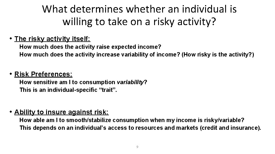
What determines whether an individual is willing to take on a risky activity? • The risky activity itself: How much does the activity raise expected income? How much does the activity increase variability of income? (How risky is the activity? ) • Risk Preferences: How sensitive am I to consumption variability? This is an individual-specific “trait”. • Ability to insure against risk: How able am I to smooth/stabilize consumption when my income is risky/variable? This depends on an individual’s access to resources and markets (credit and insurance). 9

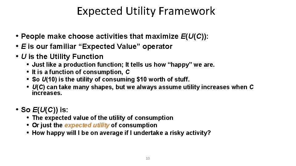
Expected Utility Framework • People make choose activities that maximize E(U(C)): • E is our familiar “Expected Value” operator • U is the Utility Function • • Just like a production function; It tells us how “happy” we are. It is a function of consumption, C So U(10) is the utility of consuming $10 worth of stuff. U(C) can take many shapes, but we always assume utility increases when C increases. • So E(U(C)) is: • The expected value of the utility of consumption • Or just the expected utility of consumption • How happy will I be on average if I undertake a risky activity? 10

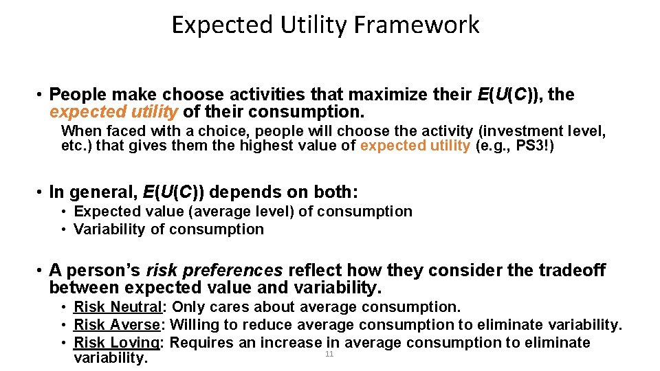
Expected Utility Framework • People make choose activities that maximize their E(U(C)), the expected utility of their consumption. When faced with a choice, people will choose the activity (investment level, etc. ) that gives them the highest value of expected utility (e. g. , PS 3!) • In general, E(U(C)) depends on both: • Expected value (average level) of consumption • Variability of consumption • A person’s risk preferences reflect how they consider the tradeoff between expected value and variability. • Risk Neutral: Only cares about average consumption. • Risk Averse: Willing to reduce average consumption to eliminate variability. • Risk Loving: Requires an increase in average consumption to eliminate 11 variability.

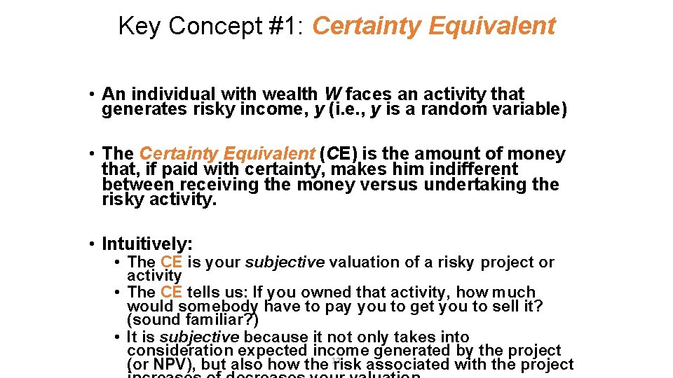
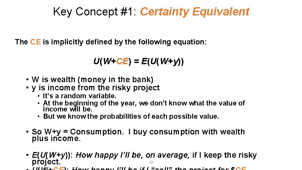
Key Concept #1: Certainty Equivalent • An individual with wealth W faces an activity that generates risky income, y (i. e. , y is a random variable) • The Certainty Equivalent (CE) is the amount of money that, if paid with certainty, makes him indifferent between receiving the money versus undertaking the risky activity. • Intuitively: • The CE is your subjective valuation of a risky project or activity • The CE tells us: If you owned that activity, how much would somebody have to pay you to get you to sell it? (sound familiar? ) • It is subjective because it not only takes into consideration expected income generated by the project 12 (or NPV), but also how the risk associated with the project

Key Concept #1: Certainty Equivalent The CE is implicitly defined by the following equation: U(W+CE) = E(U(W+y)) • W is wealth (money in the bank) • y is income from the risky project • It’s a random variable. • At the beginning of the year, we don’t know what the value of income will be. • But we know the probabilities of each possible value. • So W+y = Consumption. I buy consumption with wealth plus income. • E(U(W+y)): How happy I’ll be, on average, if I keep the risky 13 project.

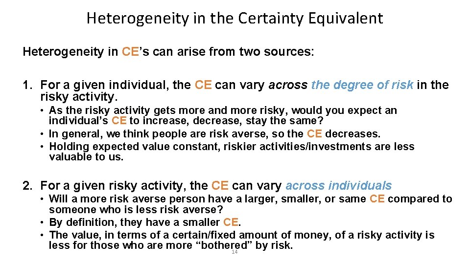
Heterogeneity in the Certainty Equivalent Heterogeneity in CE’s can arise from two sources: 1. For a given individual, the CE can vary across the degree of risk in the risky activity. • As the risky activity gets more and more risky, would you expect an individual’s CE to increase, decrease, stay the same? • In general, we think people are risk averse, so the CE decreases. • Holding expected value constant, riskier activities/investments are less valuable to us. 2. For a given risky activity, the CE can vary across individuals • Will a more risk averse person have a larger, smaller, or same CE compared to someone who is less risk averse? • By definition, they have a smaller CE. • The value, in terms of a certain/fixed amount of money, of a risky activity is less for those who are more “bothered” by risk. 14

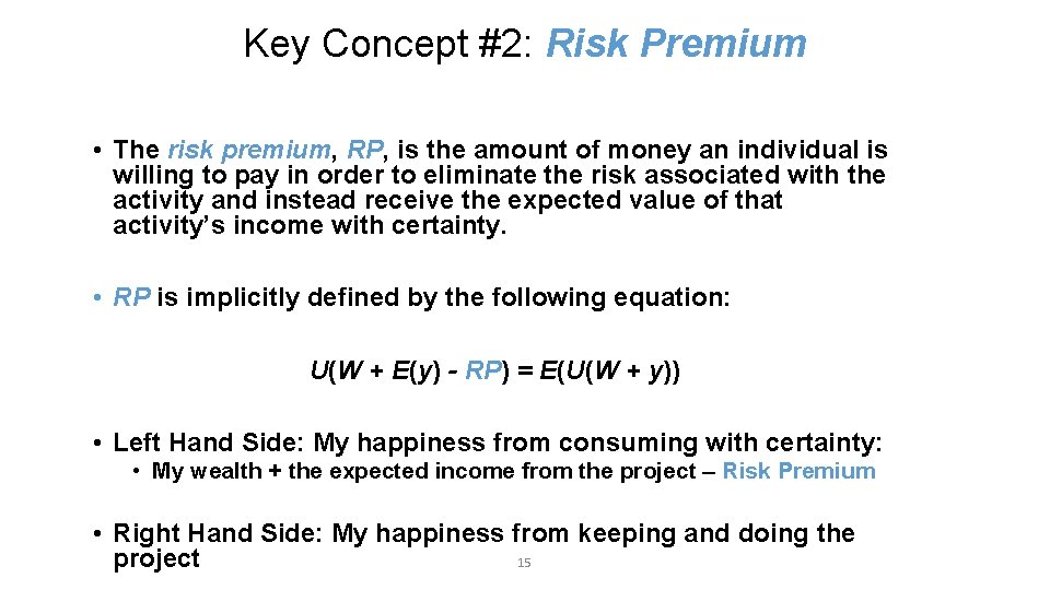
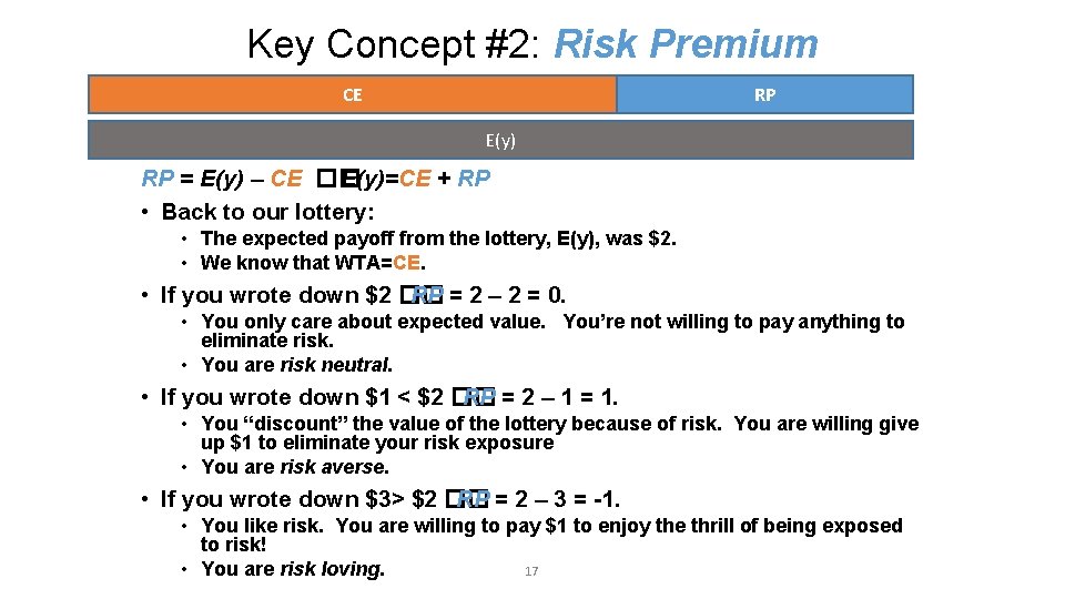
Key Concept #2: Risk Premium • The risk premium, RP, is the amount of money an individual is willing to pay in order to eliminate the risk associated with the activity and instead receive the expected value of that activity’s income with certainty. • RP is implicitly defined by the following equation: U(W + E(y) - RP) = E(U(W + y)) • Left Hand Side: My happiness from consuming with certainty: • My wealth + the expected income from the project – Risk Premium • Right Hand Side: My happiness from keeping and doing the 15 project

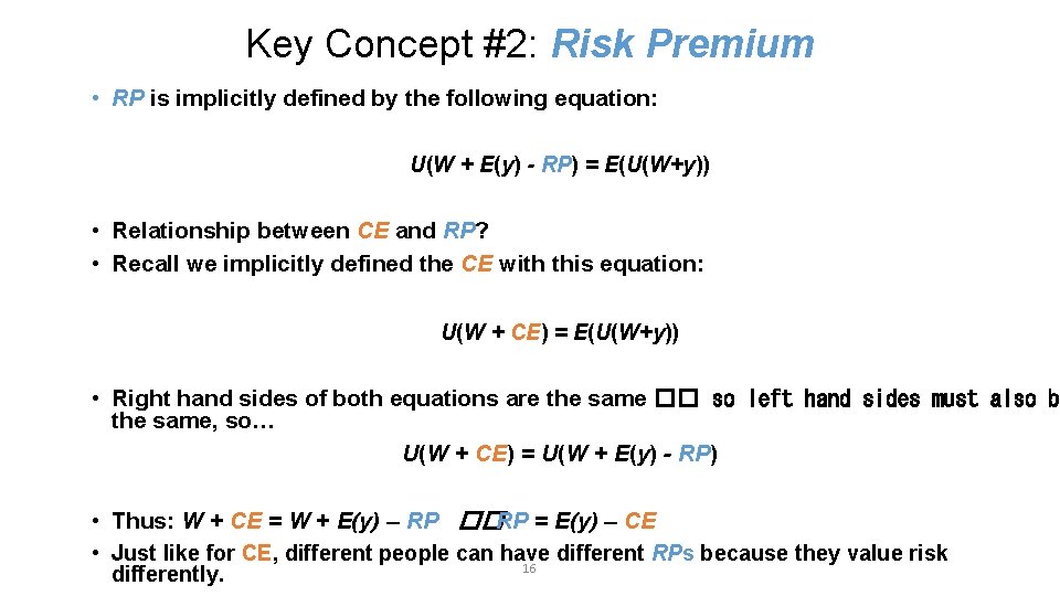
Key Concept #2: Risk Premium • RP is implicitly defined by the following equation: U(W + E(y) - RP) = E(U(W+y)) • Relationship between CE and RP? • Recall we implicitly defined the CE with this equation: U(W + CE) = E(U(W+y)) • Right hand sides of both equations are the same �� so left hand sides must also be the same, so… U(W + CE) = U(W + E(y) - RP) • Thus: W + CE = W + E(y) – RP ��RP = E(y) – CE • Just like for CE, different people can have different RPs because they value risk 16 differently.

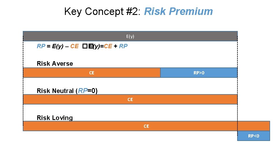
Key Concept #2: Risk Premium CE RP E(y) RP = E(y) – CE �� E(y)=CE + RP • Back to our lottery: • The expected payoff from the lottery, E(y), was $2. • We know that WTA=CE. • If you wrote down $2 �� RP = 2 – 2 = 0. • You only care about expected value. You’re not willing to pay anything to eliminate risk. • You are risk neutral. • If you wrote down $1 < $2 �� RP = 2 – 1 = 1. • You “discount” the value of the lottery because of risk. You are willing give up $1 to eliminate your risk exposure • You are risk averse. • If you wrote down $3> $2 �� RP = 2 – 3 = -1. • You like risk. You are willing to pay $1 to enjoy the thrill of being exposed to risk! 17 • You are risk loving.

Key Concept #2: Risk Premium E(y) RP = E(y) – CE �� E(y)=CE + RP Risk Averse CE RP>0 Risk Neutral (RP=0) CE Risk Loving CE RP<0

Risk Preferences • An individual is risk averse if: • RP > 0 • CE < E(y) (Since P = E(y) – CE) • They have a positive willingness to pay to eliminate risk. • An individual is risk neutral if: • RP = 0 • CE = E(y) • They are not willing to pay anything to eliminate risk -- only care about E(y). • An individual is risk loving if: • RP < 0 • CE > E(y) • They have a negative willingness to pay to eliminate their risk (they’re willing to pay to take on more risk). • In general, we believe that most people are risk averse. • What does this mean about the shape of U(C)? • See optional Canvas link to a graphical depiction of EU and risk preferences

What determines whether an individual is willing to take on a risky activity? • The risky activity itself: • How much does the activity raise expected income? • How much does the activity increase variability of income? (How risky is the activity? ) • Risk Preferences: • How sensitive am I to consumption variability? • This is an individual-specific “trait”. • Ability to insure against risk: • How able am I to smooth/stabilize consumption when my income is risky/variable? • This depends on an individual’s access to resources and markets (credit and insurance). 20

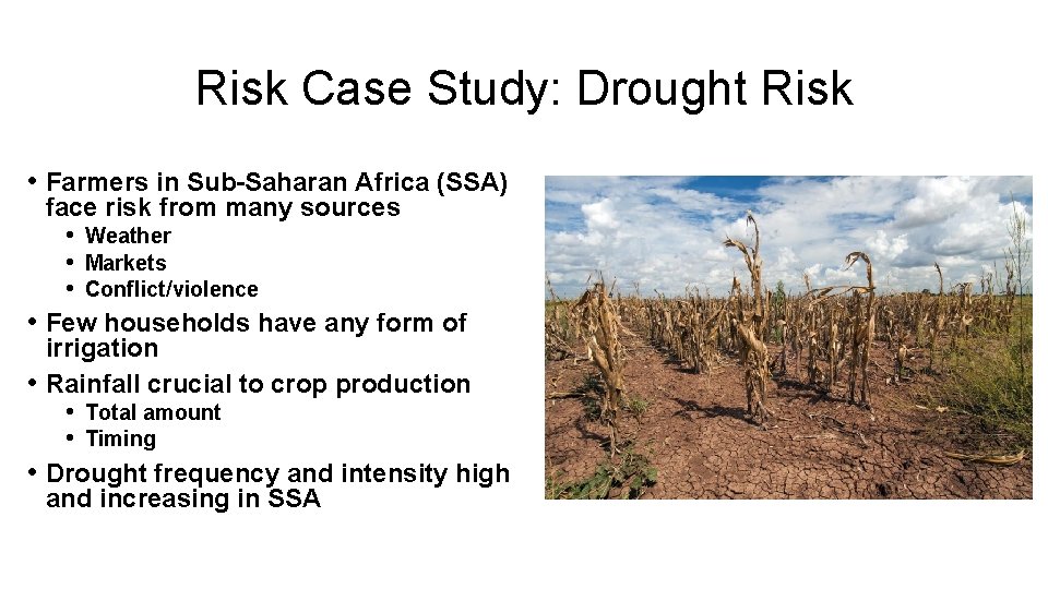
Risk Case Study: Drought Risk • Farmers in Sub-Saharan Africa (SSA) face risk from many sources • Weather • Markets • Conflict/violence • Few households have any form of irrigation • Rainfall crucial to crop production • Total amount • Timing • Drought frequency and intensity high and increasing in SSA

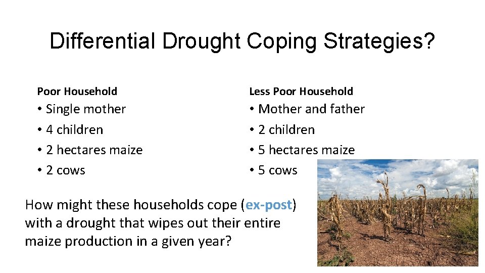
Differential Drought Coping Strategies? Poor Household Less Poor Household • Single mother • 4 children • 2 hectares maize • 2 cows • Mother and father • 2 children • 5 hectares maize • 5 cows How might these households cope (ex-post) with a drought that wipes out their entire maize production in a given year?

Differential Coping Strategies (Sidebar 12. 6) • Short run consequences of shock may be similar for different households • Farmer’s income dramatically reduced because of the drought. • Long term consequences may be very different because of different ex-post behavior (coping strategies): • Wealthier households sell off some assets to protect consumption • Poorer households protect their assets (keep the cow) and instead reduce consumption. • Why? • If poor sell assets today, they may never be able to rebuild asset stocks • Ability to generate income would be permanently weakened • So…whenever possible, hold on to productive assets and eat (even) less

Drought and Inter-generational Poverty • Protecting assets for the future by destabilizing consumption today comes at a large, long term cost for the poorest households • Recent research in SSA and elsewhere has shown that in times of drought… • • Maternal BMI declines (Hoddinot & Kinsey 2011) Growth of older children slows (later recovers) (Hoddinot & Kinsey 2011) Younger children become permanently stunted (Rochas & Soares 2015) Younger children’s long-term cognitive development damaged (Ampaabeng and Tan 2013) • Women exposed to drought as children in rural areas are poorer, shorter and less educated as adults – and their kids are more likely to be low birth weight (Hyland Russ 2019) • And yet during a drought, farmers’ kids are more likely to stay in school!?

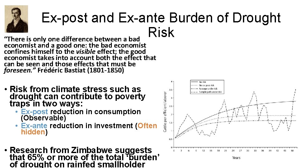
Ex-post and Ex-ante Burden of Drought Risk “There is only one difference between a bad economist and a good one: the bad economist confines himself to the visible effect; the good economist takes into account both the effect that can be seen and those effects that must be foreseen. ” Frédéric Bastiat (1801 -1850) • Risk from climate stress such as drought can contribute to poverty traps in two ways: • Ex-post reduction in consumption (Observable) • Ex-ante reduction in investment (Often hidden) • Research from Zimbabwe suggests that 65% or more of the total ‘burden’ of drought on rainfed smallholder

Drought, Activity Choice and Investment • How does this uninsured risk affect poor households’ ex-ante activity and investment choices? • Income Smoothing! • Households less likely to adopt new technologies (high yielding maize varieties) • Households less willing to invest in fertilizer • In other words, poor rural households may select lower return but less risky activities (traditional livelihoods) as a way to reduce income variability

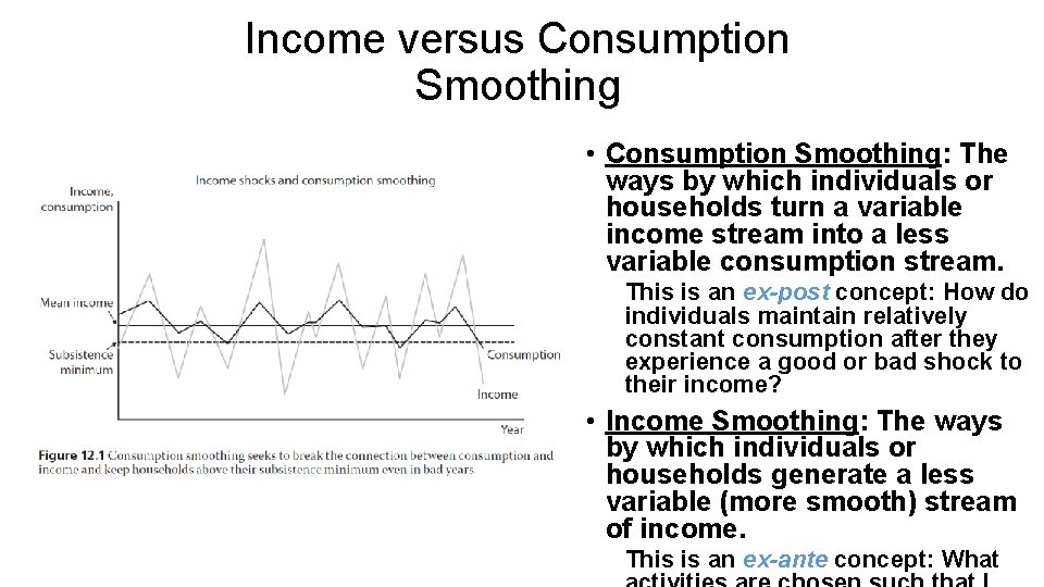
Income versus Consumption Smoothing • Consumption Smoothing: The ways by which individuals or households turn a variable income stream into a less variable consumption stream. This is an ex-post concept: How do individuals maintain relatively constant consumption after they experience a good or bad shock to their income? • Income Smoothing: The ways by which individuals or households generate a less variable (more smooth) stream of income. This is an ex-ante concept: What

Double-Whammy of Risk and Wealth • Whammy #1: Wealthy people are better able to bear risk because they have better consumption smoothing capacity. • Wealthy have more assets to sell off if they have a bad year • Credit & insurance markets tend to work better for wealthy than poor people. • Whammy #2: Wealthy people are more willing to bear risk. • Wealthier people have a lower risk premium (for a given risky activity) than poor people • Empirical evidence backs this up…risk preferences are characterized by Decreasing Absolute Risk Aversion (DARA) (risk premium for a given activity decreases as your wealth increases). • For both reasons, wealthy are more likely to do high-risk/high return activities. • Two Important Implications: Poor may be stuck in risk-induced “poverty trap” Wealth inequalities reinforced and widened over time • Implications for policy? “De-risking” the lives of the poor could unleash greater investment and productivity among the poor Why are insurance markets missing for the poor?

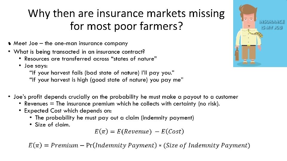
Why then are insurance markets missing for most poor farmers? •

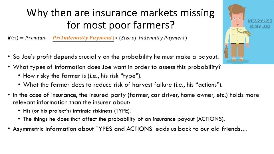
Why then are insurance markets missing for most poor farmers? •

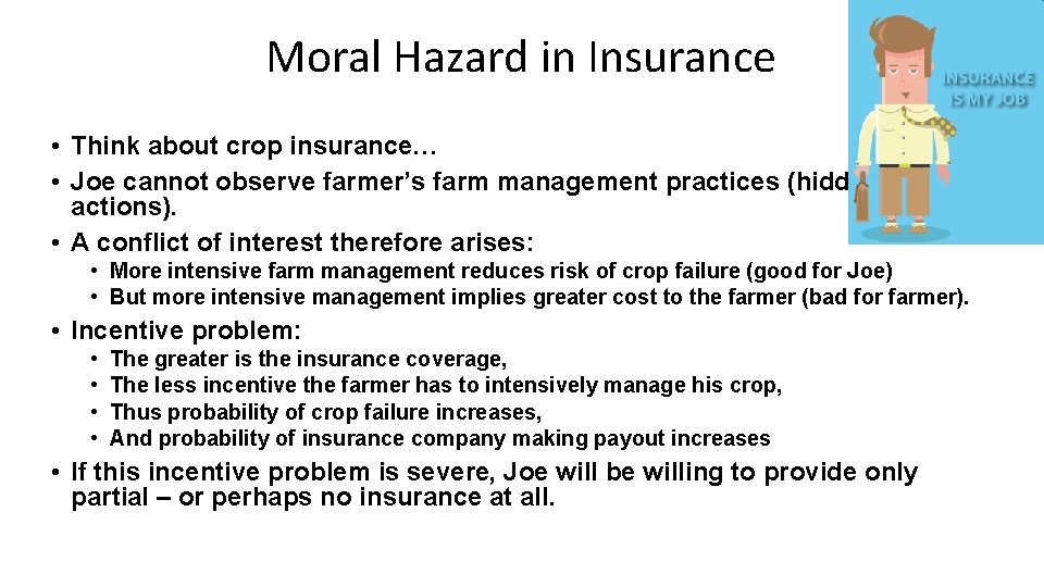
Moral Hazard in Insurance • Think about crop insurance… • Joe cannot observe farmer’s farm management practices (hidden actions). • A conflict of interest therefore arises: • More intensive farm management reduces risk of crop failure (good for Joe) • But more intensive management implies greater cost to the farmer (bad for farmer). • Incentive problem: • • The greater is the insurance coverage, The less incentive the farmer has to intensively manage his crop, Thus probability of crop failure increases, And probability of insurance company making payout increases • If this incentive problem is severe, Joe will be willing to provide only partial – or perhaps no insurance at all.

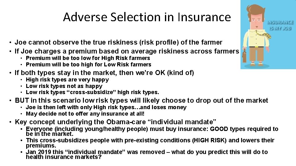
Adverse Selection in Insurance • Joe cannot observe the true riskiness (risk profile) of the farmer • If Joe charges a premium based on average riskiness across farmers then: • Premium will be too low for High Risk farmers • Premium will be too high for Low Risk farmers • If both types stay in the market, then we’re OK (kind of) • High risk types are very happy • Low risk types not as happy • Low risk types “cross-subsidize” high risk types. • BUT in this scenario low risk types will likely choose to drop out of the market • Joe is then left with only High risk types…and loses money • May decide not to offer any insurance at all! • Key concept underlying the Obama-care “individual mandate” • Everyone (including young/healthy people) must buy insurance: GOOD types required to be in the market. • This cross-subsidizes people with pre-existing conditions (HIGH RISK) and lowers their premiums. • Jan 2019 this “individual mandate” was removed – what do you predict this will do to health insurance markets?

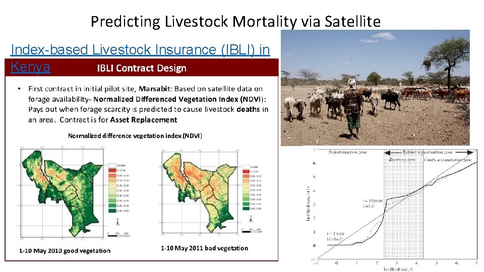
Predicting Livestock Mortality via Satellite Index-based Livestock Insurance (IBLI) in Kenya

Index Insurance: What it is and how it functions • Index insurance does not require measurement of individual losses • Instead, makes common payments to insured farmers based on the level of a single index designed to be correlated with losses. • Index insurance avoids problems that make conventional insurance unprofitable for small scale agriculture: • No transactions costs of measuring individual losses • No Moral Hazard: Preserves effort incentives as no individual can influence whether • the index pays out No Adverse Selection: Payouts do not depend on the riskiness of those who buy the insurance

So what’s the catch with Index Insurance? Basis Risk • Index insurance is only as good as the index is correlated with the losses being insured • In the case of IBLI, the NDVI index that predicts livestock mortality must be highly correlated with ACTUAL livestock mortality! • If the index is poorly designed and/or calibrated, it will be only loosely correlated with losses (or maybe not correlated at all) • The degree of correlation between the index and the losses being insured determines the Basis Risk of the index insurance • High correlation �� Low basis risk • Low correlation �� High basis risk • A “bad” IBLI index will not predict actual livestock mortality well (i. e. , low correlation), which means herders will often lose livestock and not receive an insurance payout • A “bad” index basically becomes a lottery that is disconnected from the consumption shocks a person experiences

Index Insurance: Summary • In theory, index insurance holds potential to extend formal insurance to the previously uninsurable – especially smallholders in poor countries. • Well-designed insurance can • Protect small-holders’ assets & consumption in bad years • Promote investment & technology adoption by small-holders • Increased willingness of banks to lend to small-holders • But the challenges are significant • Identifying a high quality index to minimize basis risk is difficult • Convincing insurance companies to insure farmers (let alone smallholders) is difficult • Financial literacy campaigns are required to educating farmers about insurance (which is complex!) “There are no solutions; There are only tradeoffs” Thomas Sowell