Risk Modeling of Multiyear Multiline Reinsurance Using Copulas

Risk Modeling of Multi-year, Multi-line Reinsurance Using Copulas by Ping Wang St John’s University, New York on CICIRM 2011 at Beijing, China 1

Agenda Today • Multi-year, multi-line reinsurance • A Framework Using Copulas to model time dependence • Application using real data • Concluding remarks • Q&A 2

Multi-year, multi-line reinsurance policies • Cover losses arising from multiple lines of business over multiple years (3 or 5 most common) • Stop-loss type, commonly. Reinsurer pays claims only if the accumulated losses from several business lines over an extended period exceed a fairly high threshold. • Reduced volatility compared to separate coverage 3

Difficulty Facing Actuaries • Simultaneous modeling dependence – Across time, and – Across business lines (e. g. , workers compensation and commercial multiple perils) 4

Modeling Product Risk With Copula • Assume independence between business lines • Model time-dependence of each line using copula • Simulate the distribution of future accumulated losses • Estimate the payoff of multi-year, multi-line reinsurance 5

Marginal Distribution • Suppose that there are Ti years data for a business line of the ith primary insurer • Univariate marginal distribution functions • Fit with Gamma, normal, lognormal, t-dist’n 6

Modeling Time Dependencies Using Copulas • With Copula C, the joint distribution function of Yi can be expressed as • The log-likelihood of ith primary insurer is • where c(. ) is the probability density function corresponding to the copula function • Predictive distribution is obtained based on the results of maximum likelihood estimation 7

Estimate Product Risk • Simulation of joint distribution of each business line over multiple years • Calculate the policy payoff • Analyze the risk using Va. R and CTE 8

Real Data • Loss ratios of workers compensation (WC) and commercial multiple perils (CMP) • 32 primary insurers • Task: based on the loss history of 5 years, fit the multivariate distribution, simulate the future losses, then model the risk of the reinsurance policy that covers accumulated losses of both lines over next three years. 9

Correlations across Time: WC • Loss ratios among years are not independent. WC 04 WC 03 WC 02 WC 01 WC 00 . 6483 (<. 0001) . 6640 (<. 0001) . 4611 (. 0079) . 6128 (. 0002) . 6586 (<. 0001) . 3132 (. 0809) . 3398 (. 0571) . 6144 (. 0002) . 3796 (. 0321) WC 01 . 5617 (. 0008) Reported are the value of Pearson correlations and corresponding p-values. 10

Correlations across Time: CMP 04 CMP 03 CMP 02 CMP 01 CMP 00 . 4771 (. 0058) . 3327 (. 0628) . 3200 (. 0742) . 3661 (. 0394) . 4999 (. 0036) . 1510 (. 4093) . 1225 (. 5041) . 4212 (. 0164) . 2571 (. 1554) CMP 01 . 3589 (. 0437) Reported are the value of Pearson correlations and corresponding p-values. 11

Relationship between WC & CMP • Correlation coefficient: 0. 1510 12

Fitted Marginal Distribution WC loss ratio CMP loss ratio Distribution AIC K-S stat* AIC K-S stat Lognormal 2176. 4276 0. 0383 2087. 3092 0. 0538 Gamma 2176. 0656 0. 0399 2087. 6407 0. 0709 t-dist’n 2588. 6599 0. 2707 2411. 356 0. 2561 *: kolmogorov-Smirnov test statistic 13

t-copula • t-copula: • where Gr is CDF of t-distribution function and 14

Different “correlation matrices” 15

Maximum Likelihood Estimation • Parameters to be estimated: – of copula: in correlation matrix Σ and degrees of freedom r – of marginal distribution, e. g. shape and scale parameters for Gamma 16

MLE Results: WC t-copula + Gamma margin parameter estimate Std. Error 0. 6443 Shape/mu p-value t-copula + lognormal margin estimate Std. Error p-value 0. 09136 <0. 0001 0. 6634 . 0900 <0. 0001 10. 6546 1. 9740 <0. 0001 4. 1954 0. 0455 <0. 0001 Scale/sigma 6. 6438 1. 2528 <0. 0001 0. 3235 0. 0310 <0. 0001 DF r 4. 2362 0. 2704 <0. 0001 4. 2519 0. 2704 <0. 0001 AIC 999. 77 1000. 52 17

MLE Results: CMP t-copula + Gamma margin t-copula + lognormal margin parameter estimate Std. Error p-value 0. 4339 0. 0925 <0. 0001 0. 4493 . 0947 <0. 0001 Shape/mu 11. 4205 1. 6132 <0. 0001 3. 9882 0. 0296 <0. 0001 Scale/sigma 4. 9811 0. 7206 <0. 0001 0. 3083 0. 0222 <0. 0001 DF r 4. 2524 0. 2703 <0. 0001 4. 2641 0. 2703 <0. 0001 AIC 979. 07 981. 18 18

Simulation and Analysis • Based on the multivariate distribution of the loss ratio for business lines (WC, CMP separately) for the primary insurer • Simulate the multivariate variables and • The overall loss across two lines over three years is • Where P denotes the annual premium • Payment on the reinsurance policy after deductible D 19

Histogram of Total Loss Using Different Assumptions 20

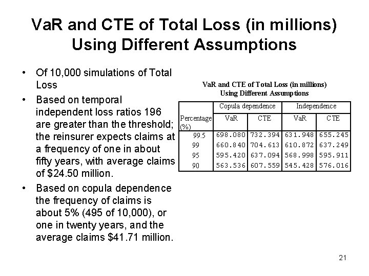
Va. R and CTE of Total Loss (in millions) Using Different Assumptions • Of 10, 000 simulations of Total Loss • Based on temporal independent loss ratios 196 are greater than the threshold; the reinsurer expects claims at a frequency of one in about fifty years, with average claims of $24. 50 million. • Based on copula dependence the frequency of claims is about 5% (495 of 10, 000), or one in twenty years, and the average claims $41. 71 million. Va. R and CTE of Total Loss (in millions) Using Different Assumptions Copula dependence Percentage (%) 99. 5 99 95 90 Independence Va. R CTE 698. 080 660. 840 595. 420 563. 536 732. 394 704. 613 637. 094 607. 559 631. 948 610. 872 568. 998 545. 428 655. 245 637. 249 595. 911 576. 016 21

Remarks • Copulas – can use information developed over time to better fit the multi-year claims experience – Can use information from similar risk classes 22

Questions and comments? Thank You! 23