Risk Management and Option Analysis Project Finance Modelling

Risk Management and Option Analysis Project Finance Modelling September 21 1

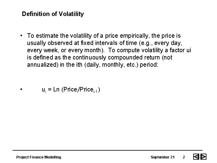
Definition of Volatility • To estimate the volatility of a price empirically, the price is usually observed at fixed intervals of time (e. g. , every day, every week, or every month). To compute volatility a factor ui is defined as the continuously compounded return (not annualized) in the ith (daily, monthly, etc. ) period: • ui = Ln (Pricei/Pricei-1) Project Finance Modelling September 21 2

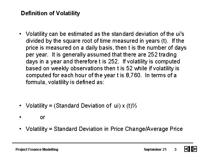
Definition of Volatility • Volatility can be estimated as the standard deviation of the ui's divided by the square root of time measured in years (t). If the price is measured on a daily basis, then t is the number of days per year. It is generally assumed that there are 252 trading days in a year and therefore t is 252. If volatility is computed based on weekly observations then t is 52 while if volatility is computed for each hour of the year t is 8, 760. In terms of a formula, volatility is defined as: • Volatility = (Standard Deviation of ui) x (t)½ • or • Volatility = Standard Deviation in Price Change/Average Price Project Finance Modelling September 21 3

Time Period for Volatility • Choosing the appropriate number of historical periods used in computing volatility is not always clear. All else being equal, more data should generally lead to better accuracy. However, volatility may change over time and old data may not be relevant for predicting the future. Furthermore, volatility may be dependent on seasonal factors -- for example volatility will probably be higher in the summer months than in the shoulder months. A rule of thumb that is often used in valuing options on stocks is to set the time period over which the volatility is measured equal to the time period over which it is to be applied. For example, if the volatility is to be used to value a two-year option, two years of historical data would be used in estimating volatility. • In measuring volatility for stock prices, time should be measured in trading days when volatility parameters are being estimated and used. In other words, days when the stock exchange is closed should be ignored for the purposes of the volatility calculation. For purposes of evaluating electricity options, if only on-peak days are applicable in exercising the option, time should be based on the number of on-peak days rather than the total number of days. If the ui is measured on an hourly basis using on-peak hours, time should be based on the number of on-peak hours in a year. Project Finance Modelling September 21 4

Time Series Equations and Risk Management • Time series equations are used to project electricity prices and other economic variables as stochastic processes, which means that a distribution of possible outcomes as well as point estimates are produced by the analysis. • By measuring a range in possible values, time series equations form the basis for risk analysis and risk management. • These equations use parameters such as: § mean reversion § trend factors § long-run equilibrium values § correlations with other prices to project • The movement from one period to the next is in part driven by random shocks. Project Finance Modelling September 21 5

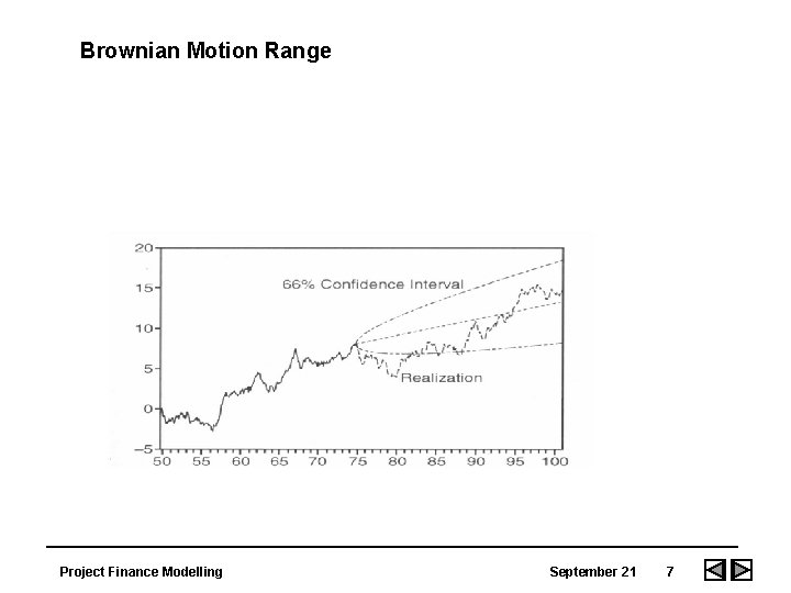
Brownian Motion • A stochastic process is a variable that evolves over time that is at least in part random. These processes are the basis for economic analysis under uncertainty. The simplest example is a random walk process where a variable can move up or down with equal probability: • Pt = Pt-1 + e. • In this equation, e is a random term that can move up or down with equal probability. In the case of Brownian motion, the e term is a draw from a normal distribution with a mean of zero and a standard deviation equal to volatility. • The price depends only on the last price and not what happened before. Brownian motion is the continuous version of the random walk. Stock prices are considered to follow this process because public information is quickly included in the current price and the past pattern has no forecasting value. If this was not the case, investors could beat the market by using past prices to predict the future. Project Finance Modelling September 21 6

Brownian Motion Range Project Finance Modelling September 21 7

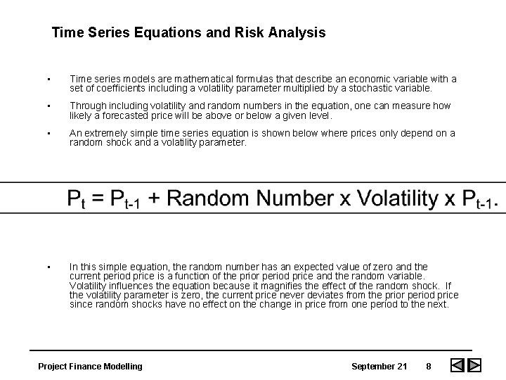
Time Series Equations and Risk Analysis • Time series models are mathematical formulas that describe an economic variable with a set of coefficients including a volatility parameter multiplied by a stochastic variable. • Through including volatility and random numbers in the equation, one can measure how likely a forecasted price will be above or below a given level. • An extremely simple time series equation is shown below where prices only depend on a random shock and a volatility parameter. • In this simple equation, the random number has an expected value of zero and the current period price is a function of the prior period price and the random variable. Volatility influences the equation because it magnifies the effect of the random shock. If the volatility parameter is zero, the current price never deviates from the prior period price since random shocks have no effect on the change in price from one period to the next. Project Finance Modelling September 21 8

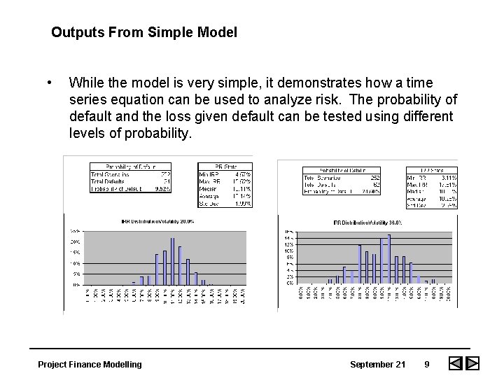
Outputs From Simple Model • While the model is very simple, it demonstrates how a time series equation can be used to analyze risk. The probability of default and the loss given default can be tested using different levels of probability. Project Finance Modelling September 21 9

Options Project Finance Modelling September 21 10

Use of Option Pricing in Project Finance • There a lot of options in project finance: § Option to develop § Option to cancel during construction § Option to operate in different ways § Option to retire plant § Option to re-finance § Credit spread as sold put option § Equity as call option Project Finance Modelling September 21 11

Option Definition • An option is the right to act on information in the future to increase value. • Standard Option Contracts • § Exercise Price § Term of the Option § Right to Exercise Call Option § • Put Option § • The right to purchase a stock at a given price at a future date. The right to sell a stock at a given price at a future date. The payoff from holding an option depends on future uncertainty and defining how the exposure to uncertainty can be limited (through defining an exercise price). Project Finance Modelling September 21 12

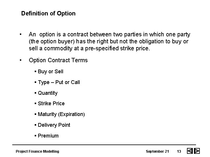
Definition of Option • An option is a contract between two parties in which one party (the option buyer) has the right but not the obligation to buy or sell a commodity at a pre-specified strike price. • Option Contract Terms § Buy or Sell § Type – Put or Call § Quantity § Strike Price § Maturity (Expiration) § Delivery Point § Premium Project Finance Modelling September 21 13

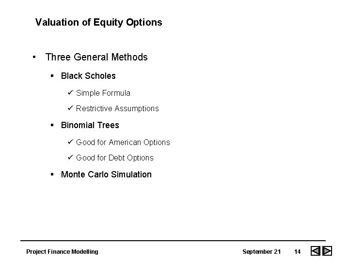
Valuation of Equity Options • Three General Methods § Black Scholes ü Simple Formula ü Restrictive Assumptions § Binomial Trees ü Good for American Options ü Good for Debt Options § Monte Carlo Simulation Project Finance Modelling September 21 14

Option Valuation • Value of payoff is equal to value cost of buying the option • Value of payoff depends on the volatility of cash flows • Measure using closed-form (Black-Scholes), Monte Carlo, or Dynamic Programming Project Finance Modelling September 21 15

Drivers of Option Value • Time Series Definition: Volatility • Time Series Definition: Mean Reversion • Risk Free Rate • Strike Price • Length of Option • Not Beta, Required Return, Growth etc. . Project Finance Modelling September 21 16

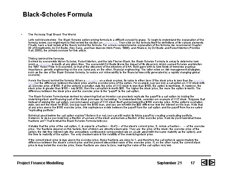
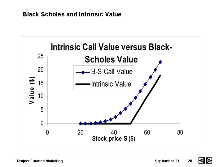
Black-Scholes Formula • The Formula That Shook The World Let's not kid ourselves: The Black-Scholes option-pricing formula is a difficult concept to grasp. To begin to understand the explanation of the formula below, you might want to first review the section on call options. Then click on the formula itself for definitions of its various elements. Finally, have a look below at theory behind the formula. For a more comprehensive explanation of the formula, we recommend Chapter 20 of Investments, by Zvi Bodie, Alex Kane, and Alan Marcus (Irwin Press, 1996), and Finance, by Zvi Bodie and Robert Merton (Prentice Hall, 2000), the primary sources for this article. Theory behind the formula Derived by economists Myron Scholes, Robert Merton, and the late Fischer Black, the Black-Scholes Formula is a way to determine how much a call option is worth at any given time. The economist Zvi Bodie likens the impact of its discovery, which earned Scholes and Merton the 1997 Nobel Prize in Economics, to that of the discovery of the structure of DNA. Both gave birth to new fields of immense practical importance: genetic engineering on the one hand and, on the other, financial engineering. The latter relies on risk-management strategies, such as the use of the Black-Scholes formula, to reduce our vulnerability to the financial insecurity generated by a rapidly changing global economy. Here's theory behind the formula: When a call option on a stock expires, its value is either zero (if the stock price is less than the exercise price) or the difference between the stock price and the exercise price of the option. For example, say you buy a call option on XYZ stock with an exercise price of $100. If at the option's expiration date the price of XYZ stock is less than $100, the option is worthless. If, however, the stock price is greater than $100 -- say $120, then the call option is worth $20. The higher the stock price, the more the option is worth. The difference between the stock price and the exercise price is the "payoff" to the call option. The Black-Scholes Formula was derived by observing that an investor can precisely replicate the payoff to a call option by buying the underlying stock and financing part of the stock purchase by borrowing. To understand this, consider our example of XYZ stock. Suppose that instead of owning the call option, you purchased a share of XYZ stock itself and borrowed the $100 exercise price. At the option's expiration date, you sell the stock for $120, you pay back the $100 loan, and you are left with the $20 difference less the interest on the loan. Note that at any price above the $100 exercise price, this equivalence exists between the payoff from the call option and the payoff from the so-called "replicating portfolio. " But what about before the call option expires? Believe it or not, you can still match its future payoff by creating a replicating portfolio. However, to do so you must buy a fraction of a share of the stock and borrow a fraction of the exercise price. How do you know what these fractions are? That is what the Black-Scholes Formula tells you. It states that the price of the call option, C, is equal to a fraction -- N(d 1) -- of the stock's current price, S, minus a fraction -- -- of the exercise price. The fractions depend on five factors, four of which are directly observable. They are: the price of the stock; the exercise price of the option; the risk-free interest rate (the annualized, continuously compounded rate on a safe asset with the same maturity as the option); and the time to maturity of the option. The only unobservable is the volatility of the underlying stock price. If the current stock price is way above the exercise price, these fractions are close to 1, and therefore the call option is approximately the difference between the stock's current price and the present discounted value of the exercise price. If, on the other hand, the current stock price is way below the exercise price, these fractions are close to zero, making the value of the call option very low. Project Finance Modelling September 21 17

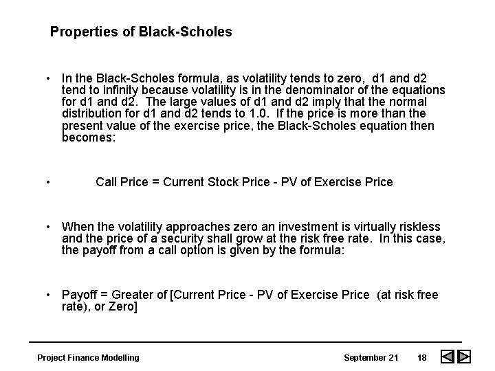
Properties of Black-Scholes • In the Black-Scholes formula, as volatility tends to zero, d 1 and d 2 tend to infinity because volatility is in the denominator of the equations for d 1 and d 2. The large values of d 1 and d 2 imply that the normal distribution for d 1 and d 2 tends to 1. 0. If the price is more than the present value of the exercise price, the Black-Scholes equation then becomes: • Call Price = Current Stock Price - PV of Exercise Price • When the volatility approaches zero an investment is virtually riskless and the price of a security shall grow at the risk free rate. In this case, the payoff from a call option is given by the formula: • Payoff = Greater of [Current Price - PV of Exercise Price (at risk free rate), or Zero] Project Finance Modelling September 21 18

Options and Arbitrage • One of the keys to option valuation is use of a risk free rate • The risk free rate derives from the fact that an option can be used to create a risk cash flow. • If the value can be boiled down to risk free cash flows, then those cash flows can be valued at the risk free rate. Project Finance Modelling September 21 19

Arbitrage • Consider cash flows from owning shares and from owing a call option. § First step: Buy some shares and sell some call options. Add the resulting cash flows in different states of the world (stock price increases and decreases) § Second step: Adjust amount of bought shares and sold options so that there is no uncertainty • The number of bought shares and sold call options gives the same cash flow whether the stock price goes up or whether it goes down § We have not put in the amount you must receive on the call option. § Since the amount is given in the future, you can invest in risk free securities. Project Finance Modelling September 21 20

Option Replication • Hedge ratio is the number of shares purchased for each call option sold or the ratio of the number of shares sold short for each call option purchased • Borrow money to pay for the shares Project Finance Modelling September 21 21

Call Option Value with No Arbitrage Profits Project Finance Modelling September 21 22

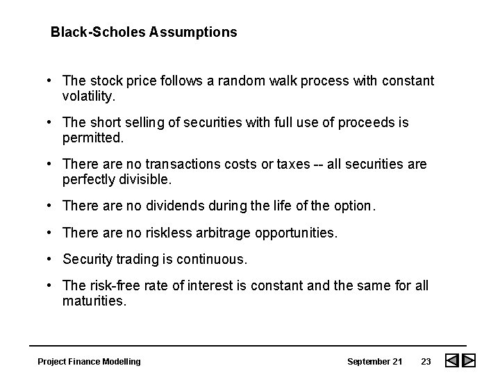
Black-Scholes Assumptions • The stock price follows a random walk process with constant volatility. • The short selling of securities with full use of proceeds is permitted. • There are no transactions costs or taxes -- all securities are perfectly divisible. • There are no dividends during the life of the option. • There are no riskless arbitrage opportunities. • Security trading is continuous. • The risk-free rate of interest is constant and the same for all maturities. Project Finance Modelling September 21 23

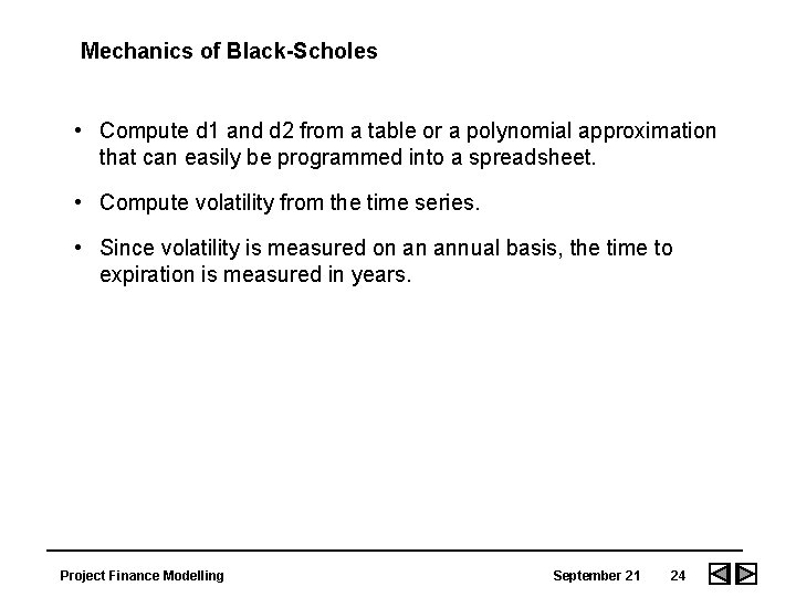
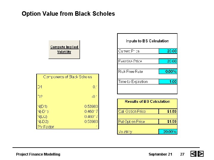
Mechanics of Black-Scholes • Compute d 1 and d 2 from a table or a polynomial approximation that can easily be programmed into a spreadsheet. • Compute volatility from the time series. • Since volatility is measured on an annual basis, the time to expiration is measured in years. Project Finance Modelling September 21 24

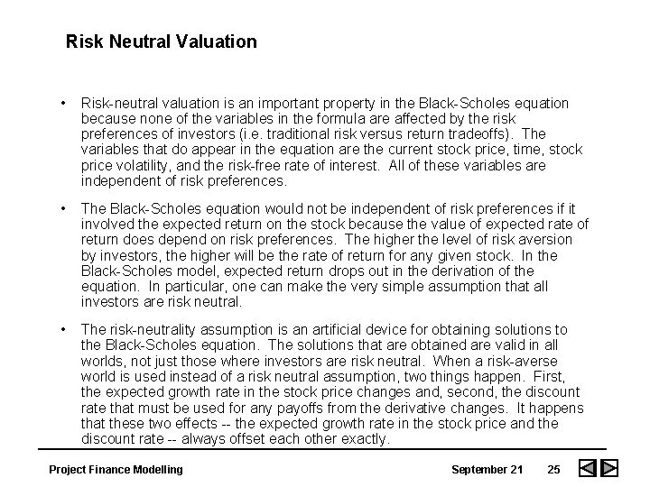
Risk Neutral Valuation • Risk-neutral valuation is an important property in the Black-Scholes equation because none of the variables in the formula are affected by the risk preferences of investors (i. e. traditional risk versus return tradeoffs). The variables that do appear in the equation are the current stock price, time, stock price volatility, and the risk-free rate of interest. All of these variables are independent of risk preferences. • The Black-Scholes equation would not be independent of risk preferences if it involved the expected return on the stock because the value of expected rate of return does depend on risk preferences. The higher the level of risk aversion by investors, the higher will be the rate of return for any given stock. In the Black-Scholes model, expected return drops out in the derivation of the equation. In particular, one can make the very simple assumption that all investors are risk neutral. • The risk-neutrality assumption is an artificial device for obtaining solutions to the Black-Scholes equation. The solutions that are obtained are valid in all worlds, not just those where investors are risk neutral. When a risk-averse world is used instead of a risk neutral assumption, two things happen. First, the expected growth rate in the stock price changes and, second, the discount rate that must be used for any payoffs from the derivative changes. It happens that these two effects -- the expected growth rate in the stock price and the discount rate -- always offset each other exactly. Project Finance Modelling September 21 25

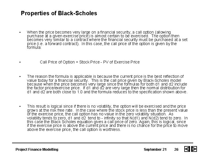
Properties of Black-Scholes • • When the price becomes very large on a financial security, a call option (allowing purchase at a given exercise price) is almost certain to be exercised. The option then becomes very similar to a contract where the financial security must be purchased at a set price (i. e. a forward contract). In this case, the call price of the option is given by the formula: Call Price of Option = Stock Price - PV of Exercise Price • The reason the formula is applicable is because the current price is the best reflection of value today for a financial security. This is the call price given by Black-Scholes model because when the price becomes very large since the formulas for both d 1 and d 2 include the factor price/exercise price. If d 1 and d 2 are very large then the normal distribution for d 1 and d 2 are both close to 1. 0 and the formula reduces to the specification shown above. • This result is logical since if there is no volatility, the option will be exercised and the price grows at the risk free rate. In the case where the stock price is less than the present value of the exercise price, the call option has no value in the zero volatility situation. As volatility tends to zero, d 1 and d 2 tend to - infinity so that N(d 1) and N(d 2) tend to zero. In this case the Black Scholes equation gives a call price of zero. Again, this is logical, since if the exercise price is above the current price and there is no chance for the price to move above the exercise price, the call option is worthless. Project Finance Modelling September 21 26

Option Value from Black Scholes Project Finance Modelling September 21 27

Black Scholes and Intrinsic Value Project Finance Modelling September 21 28

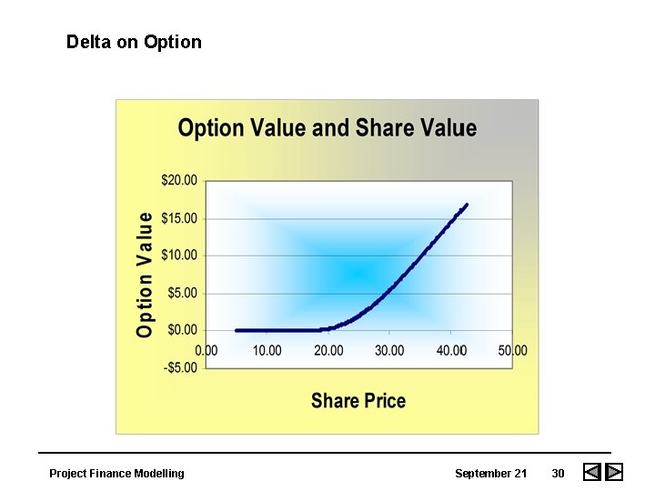
Computation of Delta, Gama, Vega and Theta • Change in the value of an option relative to the change in something else -- the stock price, the interest rate, the change in the stock price, the term to expiration • Used to in hedging to make sure that the amount of the option and the amount of the stocks are appropriate Project Finance Modelling September 21 29

Delta on Option Project Finance Modelling September 21 30

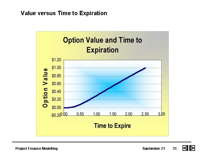
Value versus Time to Expiration Project Finance Modelling September 21 31

Other Greeks • Gamma - The change in delta resulting from a change in stock price • Theta - Change in option value as time to expiration changes • Kappa - Change in option value as volatility changes • Lambda - Change in option value as interest rate changes Project Finance Modelling September 21 32

Time Series Models Project Finance Modelling September 21 33

Economic Assumptions and Time Series Analysis • Time series analysis is an effective way to discuss modeling of economic assumptions. The next slide illustrates how a time series model works. Some issues related to time series models include: § Commodity prices very often are directly or indirectly drive value § Time series analysis is important because risk is driven by the variability in commodity prices (mcarlo. xls) § Volatility and other parameters can be gauged through implied data from financial markets, statistical analysis and economic concepts § Project finance requires long-term assessment of time series parameters Project Finance Modelling September 21 34

Time Series Models • Practical Notes: § Models such as random walk built for relatively short-term analysis rather than 20 -30 year investment decisions ü Review results to make sure they make sense in the long-run ü Compute the resulting volatility, correlation and mean reversion from the models. ü Think about the economic drivers of volatility, mean reversion, price boundaries and correlation. Project Finance Modelling September 21 35

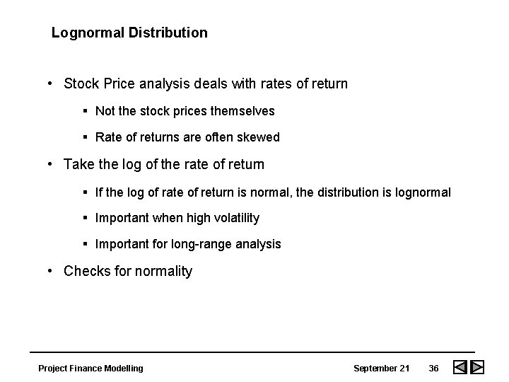
Lognormal Distribution • Stock Price analysis deals with rates of return § Not the stock prices themselves § Rate of returns are often skewed • Take the log of the rate of return § If the log of rate of return is normal, the distribution is lognormal § Important when high volatility § Important for long-range analysis • Checks for normality Project Finance Modelling September 21 36

Value at Risk • Lower tail value for a portfolio below which there is a KNOWN chance that the asset will fall. • Attempt to measure the downside risk of an asset with a single number – the maximum loss at a given percentile for a given time period. • Translate from volatility to the appropriate percentile of a normal distribution • With a standard normal distribution, there is a 5% chance of being 1. 64 standard deviations or more below the mean. • 2. 5% chance of 1. 96 standard deviations below the mean. Project Finance Modelling September 21 37

Time Series Models - Teaching Objectives • Economic theory behind alternative time series models • Brownian motion time series • Mean reversion time series • Jump process time series • Use of alternative time series in assumption development of financial models Project Finance Modelling September 21 38

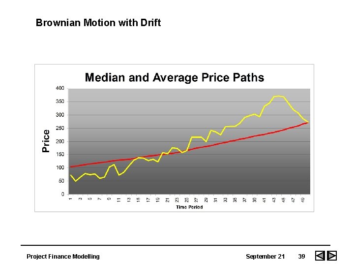
Brownian Motion with Drift Project Finance Modelling September 21 39

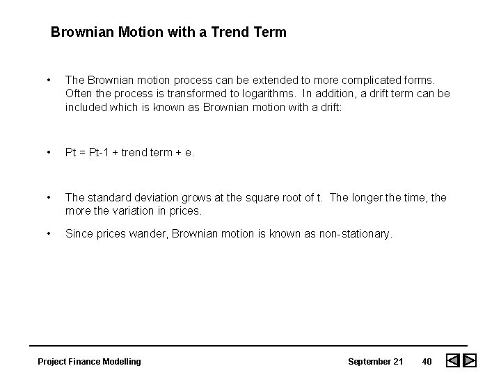
Brownian Motion with a Trend Term • The Brownian motion process can be extended to more complicated forms. Often the process is transformed to logarithms. In addition, a drift term can be included which is known as Brownian motion with a drift: • Pt = Pt-1 + trend term + e. • The standard deviation grows at the square root of t. The longer the time, the more the variation in prices. • Since prices wander, Brownian motion is known as non-stationary. Project Finance Modelling September 21 40

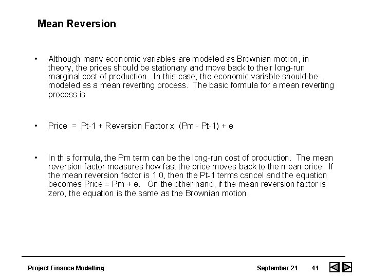
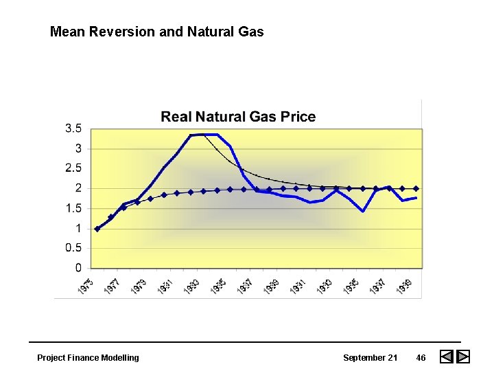
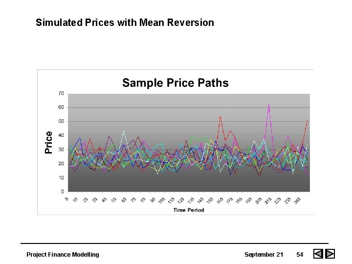
Mean Reversion • Although many economic variables are modeled as Brownian motion, in theory, the prices should be stationary and move back to their long-run marginal cost of production. In this case, the economic variable should be modeled as a mean reverting process. The basic formula for a mean reverting process is: • Price = Pt-1 + Reversion Factor x (Pm - Pt-1) + e • In this formula, the Pm term can be the long-run cost of production. The mean reversion factor measures how fast the price moves back to the mean price. If the mean reversion factor is 1. 0, then the Pt-1 terms cancel and the equation becomes Price = Pm + e. On the other hand, if the mean reversion factor is zero, the equation is the same as the Brownian motion. Project Finance Modelling September 21 41

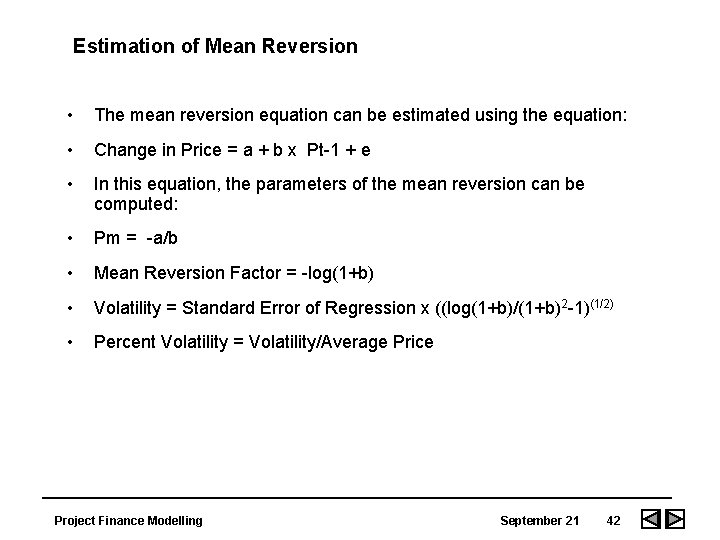
Estimation of Mean Reversion • The mean reversion equation can be estimated using the equation: • Change in Price = a + b x Pt-1 + e • In this equation, the parameters of the mean reversion can be computed: • Pm = -a/b • Mean Reversion Factor = -log(1+b) • Volatility = Standard Error of Regression x ((log(1+b)/(1+b)2 -1)(1/2) • Percent Volatility = Volatility/Average Price Project Finance Modelling September 21 42

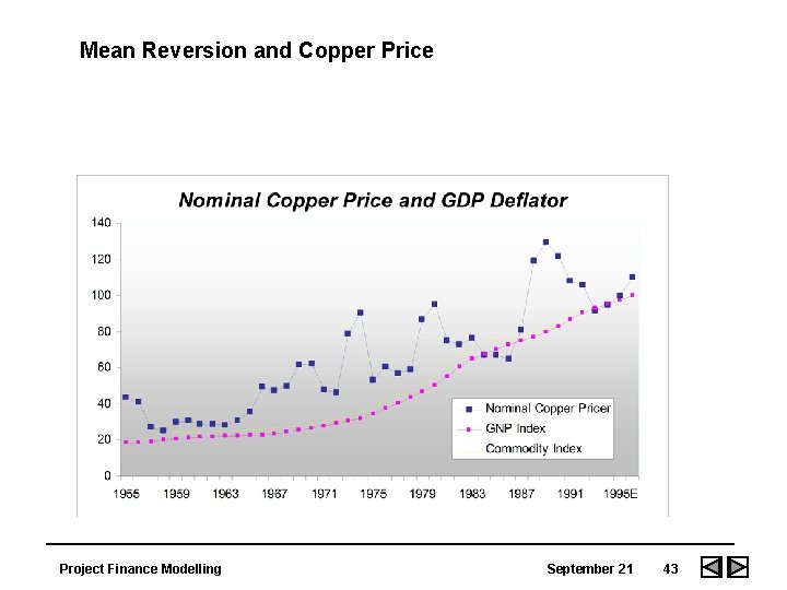
Mean Reversion and Copper Price Project Finance Modelling September 21 43

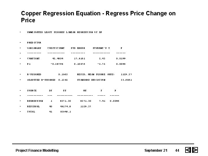
Copper Regression Equation - Regress Price Change on Price • UNWEIGHTED LEAST SQUARES LINEAR REGRESSION OF DP • PREDICTOR • VARIABLES COEFFICIENT STD ERROR STUDENT'S T P • ----------- ------ • CONSTANT • P 1 • R-SQUARED 0. 1563 RESID. MEAN SQUARE (MSE) 1129. 37 • ADJUSTED R-SQUARED 0. 1352 STANDARD DEVIATION 33. 6061 • SOURCE • 42. 4804 17. 5161 2. 43 0. 0199 -0. 28795 0. 10576 -2. 72 0. 0096 DF SS MS F P ---------- ------ • REGRESSION 1 8371. 30 7. 41 0. 0096 • RESIDUAL 40 45174. 8 1129. 37 • TOTAL 41 53546. 1 Project Finance Modelling September 21 44

Boundary Conditions • Lower bound is short-term marginal cost. • Upper bound can be driven by regulatory requirements. • Trend factor is driven by productivity improvements. Project Finance Modelling September 21 45

Mean Reversion and Natural Gas Project Finance Modelling September 21 46

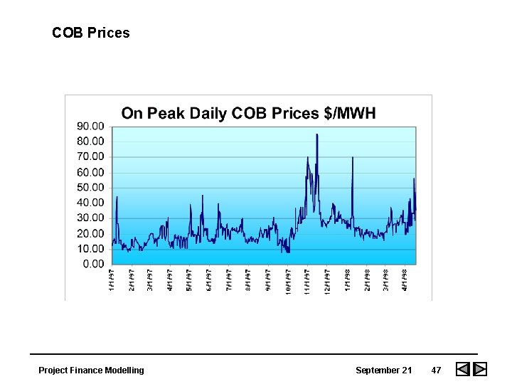
COB Prices Project Finance Modelling September 21 47

• Monte Carlo Simulation of Time Series Project Finance Modelling September 21 48

Simulation • Objective of simulation is to mathematically measure risk. • Monte Carlo simulation and is relevant where true options exist. In other cases, simulation can be over-used. • Simulation in project finance combines time series analysis with the basic project finance model (simulate). Project Finance Modelling September 21 49

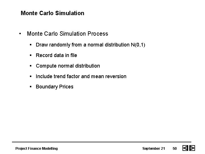
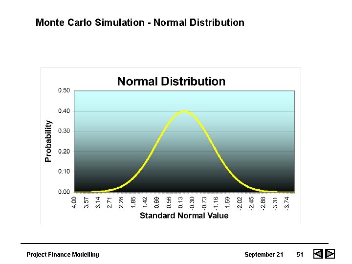
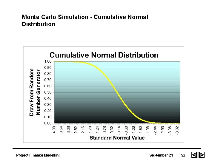
Monte Carlo Simulation • Monte Carlo Simulation Process § Draw randomly from a normal distribution N(0, 1) § Record data in file § Compute normal distribution § Include trend factor and mean reversion § Boundary Prices Project Finance Modelling September 21 50

Monte Carlo Simulation - Normal Distribution Project Finance Modelling September 21 51

Monte Carlo Simulation - Cumulative Normal Distribution Project Finance Modelling September 21 52

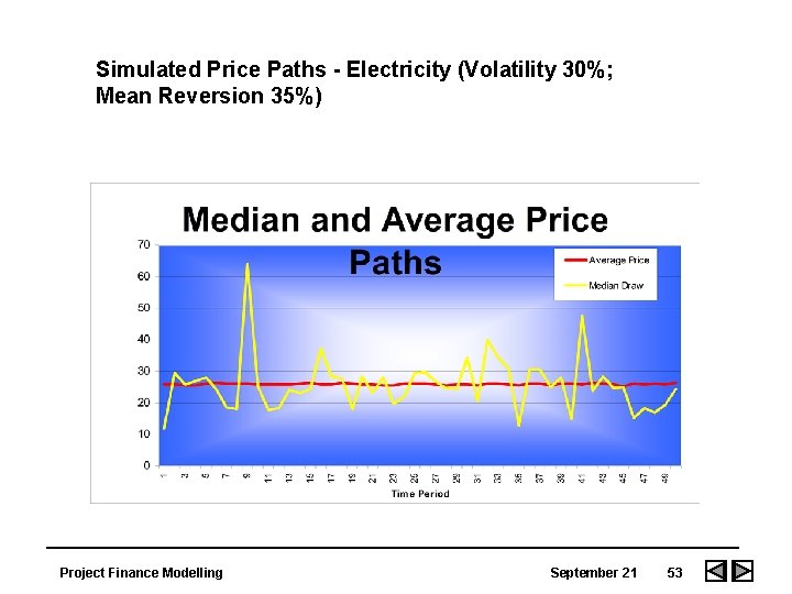
Simulated Price Paths - Electricity (Volatility 30%; Mean Reversion 35%) Project Finance Modelling September 21 53

Simulated Prices with Mean Reversion Project Finance Modelling September 21 54

Problem with Time Series • Where everything works according to the law of probability, we are like primitive people or gamblers -- who have no recourse but to recant incantations to our gods. Nothing we do, no judgement we make … is going to have the slightest influence on the final result. Project Finance Modelling September 21 55

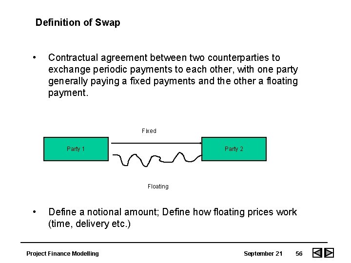
Definition of Swap • Contractual agreement between two counterparties to exchange periodic payments to each other, with one party generally paying a fixed payments and the other a floating payment. Fixed Party 1 Party 2 Floating • Define a notional amount; Define how floating prices work (time, delivery etc. ) Project Finance Modelling September 21 56