RIP Alex http youtube comwatch vs Ykw E

RIP Alex: http: //youtube. com/watch? v=s. Yk-w. E 18 BTo Local Search & CSP 1. Homework 2 socket opened 2. How is project going? 3. No class on Monday

Search when states are factored • Until now, we assumed states are blackboxes. • We will now assume that states are made up of “state-variables” and their “values” • Two interesting problem classes – CSP & SAT (Constraint Satisfaction Problems) – Planning
 X Red green blue X Y Z")
Constraint Satisfaction Problems (a brief animated overview) X Red green blue X Y Z Coloring Problem Red green blue • Search backtracking, variable/value heuristics Red green blue Y Z Constraint Graph • Inference Consistency enforcement, forward checking X: red Y: blue Z: green Variables Problem Statement Values CSP Algorithm Solution Constraints CSP Representation December 2, 1998 Sqalli, Tutorial on Constraint Satisfaction Problems 3

Other examples of CSP problems. . • Most assignment problems including – Time-tabling • Variables: Courses; Values: Rooms, times – Jobshop Scheduling • Variables: jobs; values: machines • Sudoku • Cross-word puzzle • Boolean satisfiability

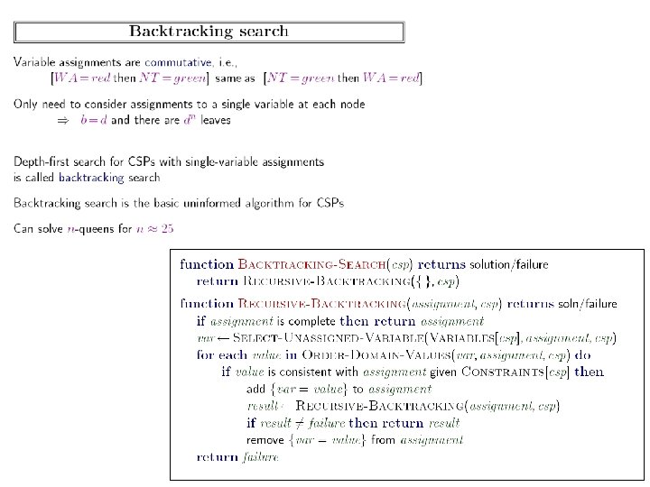
General Search vs. CSP • • Blackbox State External Child-generator State-space can be infinite External goal test Goals can occur at any depth Goals can have different costs All the search algorithms we discussed until now are appropriate. Heuristics are aimed at estimating the cost to goal node. . • • • State is made-up of state variables Children generation involves assigning values to more variables State space is finite A state is a goal state if all variables are assigned and no constraints are violated All goals occur at the same depth In the basic formulation, all goals have the same cost – This can be generalized • • Only the Depth-first search makes sense! Heuristics are aimed at picking the right variable to assign next, and deciding the right value to assign to it.

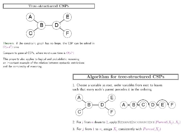
Complexity of CSP. . • Boolean Satisfiability is a special case of discrete variable CSP problem – So, CSP is NP-hard • Specific types of CSP may be tractable. – E. g. if all the variables are boolean and all the constraints are binary, you have 2 -SAT which is tractable. – The topology of the “constraint graph” also affects the complexity of the CSP problem • E. g. If the constraint graph is a chain graph or a multi-tree, we can solve it polynomially


Review of CSP/SAT concepts x, y, u, v: {A, B, C, D, E} w: {D, E} l : {A, B} x=A w E y=B u D u=C l A v=D l B • Constraint Satisfaction Problem (CSP) – Given • A set of variables – (Normally, discrete—but can be continuous) • Legal domains for each of the variables • A set of constraints on values groups of variables can take A solution: x=B, y=C, u=D, v=E, w=D, l=B x¬A N 1: {x=A} y¬ B – Constraints can be “Unary”, “binary” or “multi-ary” based on how many variables they connect N 2: {x= A & y = B } v¬ D N 3: {x= A & y = B & v = D } u¬ C – Find an assignment of values to all the N : {x= A & y = B & v = D & u = C } w¬ E variables so that none of the w¬ D N : {x= A & y = B & v = D & u = C & w= E } constraints are violated N : {x= A & y = B & v = D & u = C & w= D } • SAT Problem = CSP with boolean variables 4 5 6


“Most Constrained Variable First” “Least-constraining Value First”

y n n n y Dynamic variable ordering: Pick the variable with the smallest “live” (remaining) domain next.

“Electric Justice: US-Style” Just another day in the university. . 9/19

Constraint Graphs will be hyper-graphs for non-binary CSPs

Things discussed on board • If the constraint graph is disconnected, then you essentially have independent subproblems. – For example, suppose you mixed up a coloring problem CSP with a queens problm CSP • • You are better off solving them separately and concatenating the results You may ask “Why should I solve them separately? Can’t my search algorithm find the independence itself? – The answer is that normal search algorithms that do chronological backtracking are unable to recognize and exploit problem independence dynamically. – You need “dependency directed backtracking” • Another question is how to do constraint graphs when you have non-binary (ternary etc. ) constraints – When you have n-ary (n>2) constraints, your constraint graph is a hyper graph (with edges connecting a set rather than a pair of vertices) – It is possible to convert every non-binary CSP into a binary CSP (by introducing new variables. If there is a constraint between X, Y, and Z, I can introduce a super variable called x-y and make a binary constraint between it and Z) • Of course, when you do this, the resulting constraints may not be natural for someone who knows the domain – • Just as an assembly language program may not make as much sense to a domain expert as does a high-level language program Binary CSPs and Boolean CSPs are canonical classes of CSP in that any arbitrary CSP can be “compiled down” to an equivalent binary or boolean CSP

Not enough to show the correct configuration of the 18 -puzzle problem or rubik’s cube. . (although by including the list of actions as part of the state, you can support hill-climbing)

What is needed: --A neighborhood function The larger the neighborhood you consider, the less myopic the search (but the more costly each iteration) --A “goodness” function needs to give a value to non-solution configurations too for 8 queens: (-ve) of number of pair-wise conflicts
 be the")
A greedier version of the above: For each variable v, let l(v) be the value that it can take so that the number of conflicts are minimized. Let n(v) be the number of conflicts with this value. --Pick the variable v with the lowest n(v) value. --Assign it the value l(v) 2 1 This one basically searches the 1 -neighborhood of the current assignment (where k-neighborhood is all assignments that differ from the current assignment in atmost k-variable values) I pointed out that The neighborhood 1 is subsumed by Neighborhood 2

Understand the tradeoffs in defining smaller vs. larger neighborhood Applying min-conflicts based hill-climbing to 8 -puzzle Local Minima
: Random restart hill-climbing Do the non-greedy thing with some")
Problematic scenarios for hill-climbing Solution(s): Random restart hill-climbing Do the non-greedy thing with some probability p>0 Use simulated annealing Ridges When the state-space landscape has local minima, any search that moves only in the greedy direction cannot be (asymptotically) complete Random walk, on the other hand, is asymptotically complete Idea: Put random walk into greedy hill-climbing

Ideas for improving convergence: -- Random restart hill-climbing After every N iterations, start with a completely random assignment --Probabilistic greedy -with probability p do what the greedy strategy suggests -with probability (1 -p) pick a random variable and change its value randomly -- p can increase as the search A greedier version of the above: progresses For each variable v, let l(v) be the value that it can take so that the number of conflicts are minimized. Let n(v) be the number of conflicts with this value. --Pick the variable v with the lowest n(v) value. --Assign it the value l(v) 2 1 This one basically searches the 1 -neighborhood of the current assignment (where k-neighborhood is all assignments that differ from the current assignment in atmost k-variable values) I pointed out that The neighborhood 1 is subsumed by Neighborhood 2

Making Hill-Climbing Asymptotically Complete • Random restart hill-climbing – Keep some bound B. When you made more than B moves, reset the search with a new random initial seed. Start again. • Getting random new seed in an implicit search space is non-trivial! – In 8 -puzzle, if you generate a random state by making random moves from current state, you are still not truly random (as you will continue to be in one of the two components) • “biased random walk”: Avoid being greedy when choosing the seed for next iteration – With probability p, choose the best child; but with probability (1 -p) choose one of the children randomly • Use simulated annealing – Similar to the previous idea—the probability p itself is increased asymptotically to one (so you are more likely to tolerate a nongreedy move in the beginning than towards the end) With random restart or the biased random walk strategies, we can solve very large problems million queen problems in under minutes!

AT 3 -S e. T s Pha ion sit ran ~4. 3 #clauses / # Variables

--didn’t discuss the remaining slides--

The middle ground between hill-climbing and systematic search • Hill-climbing has a lot of freedom in deciding which node to expand next. But it is incomplete even for finite search spaces. – Good for problems which have solutions, but the solutions are non-uniformly clustered. • Systematic search is complete (because its search tree keeps track of the parts of the space that have been visited). – Good for problems where solutions may not exist, • Or the whole point is to show that there are no solutions (e. g. propositional entailment problem to be discussed later). – or the state-space is densely connected (making repeated exploration of states a big issue). Smart idea: Try the middle ground between the two?

Between Hill-climbing and systematic search • You can reduce the freedom of hillclimbing search to make it more complete – Tabu search • You can increase the freedom of systematic search to make it more flexible in following local gradients – Random restart search

Random restart search Variant of depth-first search where • When a node is expanded, its children are first randomly permuted before being introduced into the open list – The permutation may well be a “biased” random permutation • Search is “restarted” from scratch anytime a “cutoff” parameter is exceeded – There is a “Cutoff” (which may be in terms of # of backtracks, #of nodes expanded or amount of time elapsed) • Because of the “random” permutation, every time the search is restarted, you are likely to follow different paths through the search tree. This allows you to recover from the bad initial moves. • The higher the cutoff value the lower the amount of restarts (and thus the lower the “freedom” to explore different paths). • When cutoff is infinity, random restart search is just normal depth-first search—it will be systematic and complete • For smaller values of cutoffs, the search has higher freedom, but no guarantee of completeness • A strategy to guarantee asymptotic completeness: • Start with a low cutoff value, but keep increasing it as time goes on. • Random restart search has been shown to be very good for problems that have a reasonable percentage of “easy to find” solutions (such problems are said to exhibit “heavy-tail” phenomenon). Many real-world problems have this property.
- Slides: 31