Rigid Registration Ziv Yaniv Ph D Office of

Rigid Registration Ziv Yaniv, Ph. D. , Office of High Performance Computing and Communication, National Library of Medicine, National Institutes of Health and TAJ Technologies Inc.

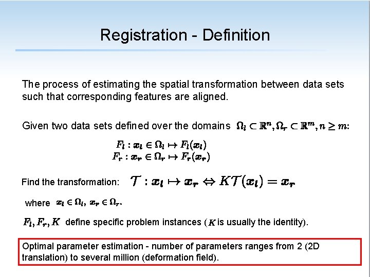
Registration - Definition The process of estimating the spatial transformation between data sets such that corresponding features are aligned. Given two data sets defined over the domains Find the transformation: where define specific problem instances ( is usually the identity). Optimal parameter estimation - number of parameters ranges from 2 (2 D translation) to several million (deformation field).

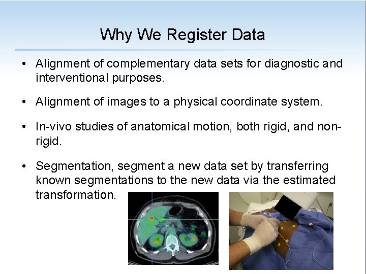
Why We Register Data • Alignment of complementary data sets for diagnostic and interventional purposes. • Alignment of images to a physical coordinate system. • In-vivo studies of anatomical motion, both rigid, and nonrigid. • Segmentation, segment a new data set by transferring known segmentations to the new data via the estimated transformation.

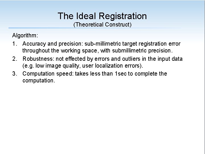
The Ideal Registration (Theoretical Construct) Algorithm: 1. Accuracy and precision: sub-millimetric target registration error throughout the working space, with submillimetric precision. 2. Robustness: not effected by errors and outliers in the input data (e. g. low image quality, user localization errors). 3. Computation speed: takes less than 1 sec to complete the computation.

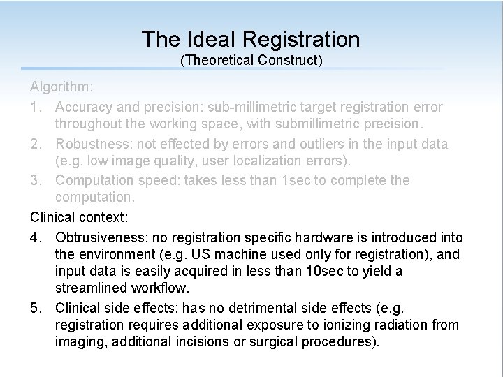
The Ideal Registration (Theoretical Construct) Algorithm: 1. Accuracy and precision: sub-millimetric target registration error throughout the working space, with submillimetric precision. 2. Robustness: not effected by errors and outliers in the input data (e. g. low image quality, user localization errors). 3. Computation speed: takes less than 1 sec to complete the computation. Clinical context: 4. Obtrusiveness: no registration specific hardware is introduced into the environment (e. g. US machine used only for registration), and input data is easily acquired in less than 10 sec to yield a streamlined workflow. 5. Clinical side effects: has no detrimental side effects (e. g. registration requires additional exposure to ionizing radiation from imaging, additional incisions or surgical procedures).

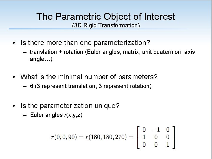
The Parametric Object of Interest (3 D Rigid Transformation) • Is there more than one parameterization? – translation + rotation (Euler angles, matrix, unit quaternion, axis angle…) • What is the minimal number of parameters? – 6 (3 represent translation, 3 represent rotation) • Is the parameterization unique? – Euler angles r(x, y, z)

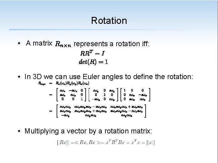
Rotation • A matrix represents a rotation iff: • In 3 D we can use Euler angles to define the rotation: • Multiplying a vector by a rotation matrix:

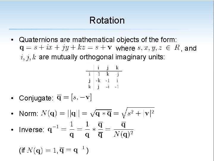
Rotation • Quaternions are mathematical objects of the form: where , and are mutually orthogonal imaginary units: • Conjugate: • Norm: • Inverse: (if , )

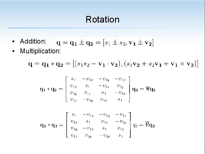
Rotation • Addition: • Multiplication:

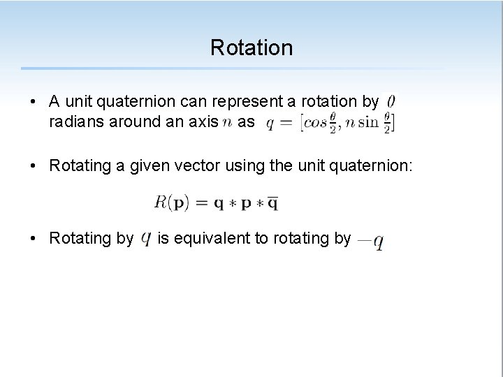
Rotation • A unit quaternion can represent a rotation by radians around an axis as • Rotating a given vector using the unit quaternion: • Rotating by is equivalent to rotating by

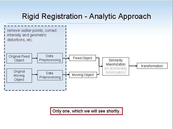
Rigid Registration - Analytic Approach remove outlier points, correct intensity and geometric distortions, etc. Original Fixed Object Original Moving Object Data Preprocessing Fixed Object Moving Object Similarity Maximization (or dissimilarity minimization) Only one, which we will see shortly. transformation

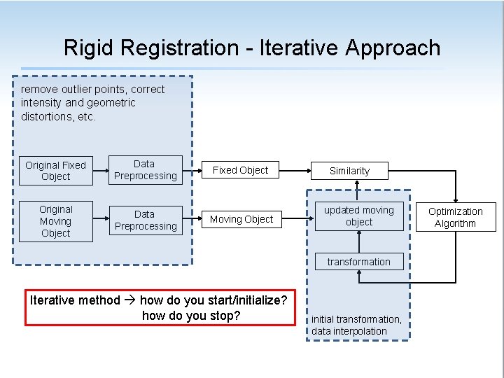
Rigid Registration - Iterative Approach remove outlier points, correct intensity and geometric distortions, etc. Original Fixed Object Data Preprocessing Fixed Object Original Moving Object Data Preprocessing Moving Object Similarity updated moving object transformation Iterative method how do you start/initialize? how do you stop? initial transformation, data interpolation Optimization Algorithm

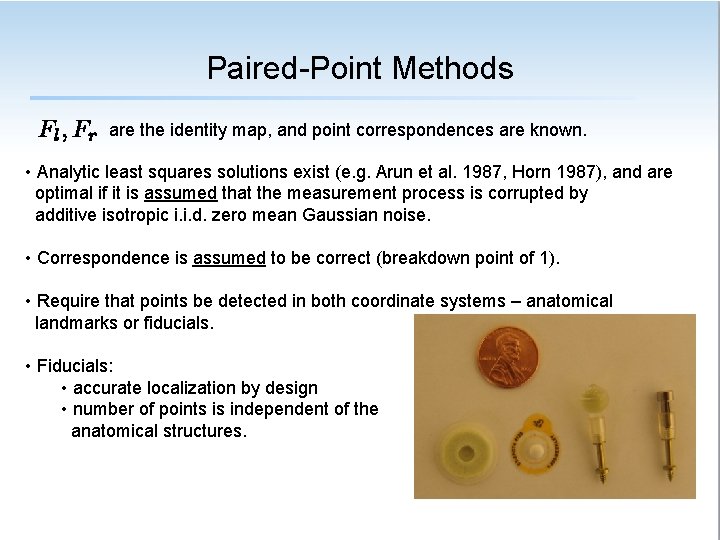
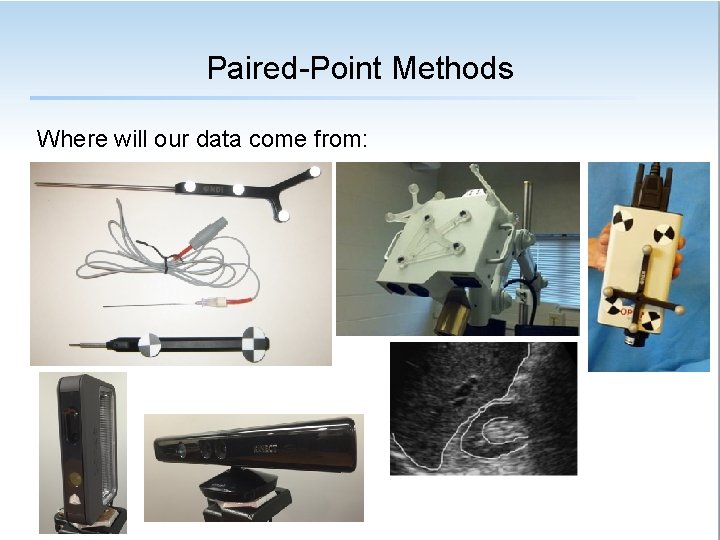
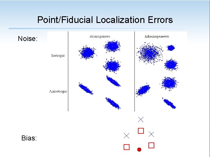
Paired-Point Methods are the identity map, and point correspondences are known. • Analytic least squares solutions exist (e. g. Arun et al. 1987, Horn 1987), and are optimal if it is assumed that the measurement process is corrupted by additive isotropic i. i. d. zero mean Gaussian noise. • Correspondence is assumed to be correct (breakdown point of 1). • Require that points be detected in both coordinate systems – anatomical landmarks or fiducials. • Fiducials: • accurate localization by design • number of points is independent of the anatomical structures.

Paired-Point Methods Where will our data come from:

Point/Fiducial Localization Errors Noise: Bias:

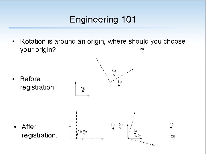
Engineering 101 • Rotation is around an origin, where should you choose your origin? • Before registration: • After registration:

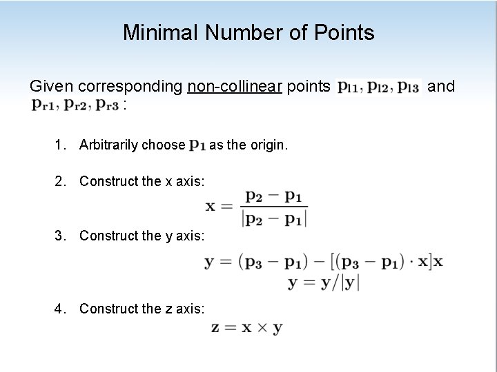
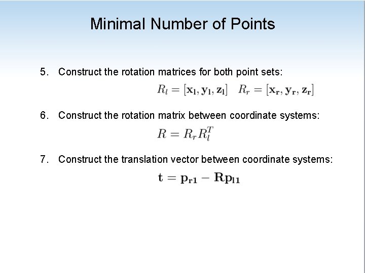
Minimal Number of Points Given corresponding non-collinear points : 1. Arbitrarily choose 2. Construct the x axis: 3. Construct the y axis: 4. Construct the z axis: as the origin. and

Minimal Number of Points 5. Construct the rotation matrices for both point sets: 6. Construct the rotation matrix between coordinate systems: 7. Construct the translation vector between coordinate systems:

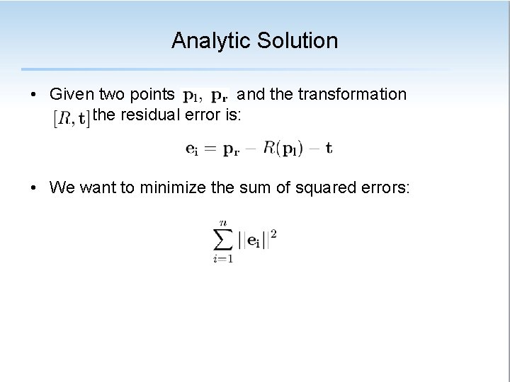
Analytic Solution • Given two points and the transformation the residual error is: • We want to minimize the sum of squared errors:

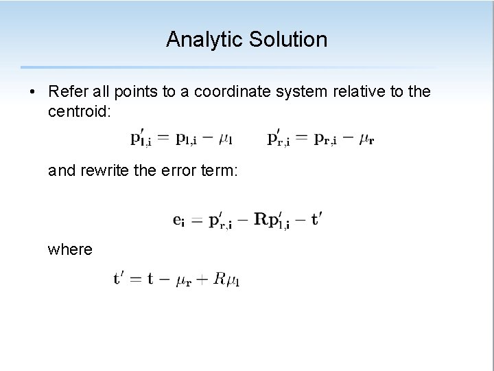
Analytic Solution • Refer all points to a coordinate system relative to the centroid: and rewrite the error term: where

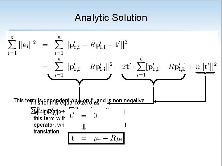
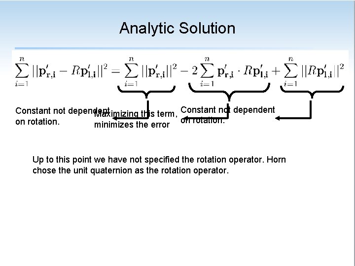
Analytic Solution This term dependent on t’, as and is non negative. Thisisterm is equalonly to zero Minimization is reduced to minimizing this term with respect to the rotation operator, which will define the optimal translation.

Analytic Solution Constant not dependent Maximizing this term, Constant not dependent on rotation. minimizes the error on rotation. Up to this point we have not specified the rotation operator. Horn chose the unit quaternion as the rotation operator.

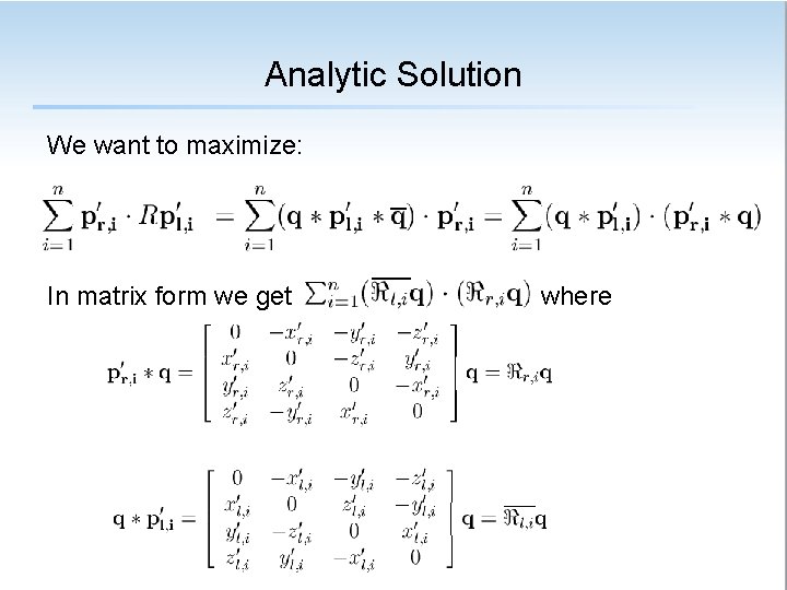
Analytic Solution We want to maximize: In matrix form we get where

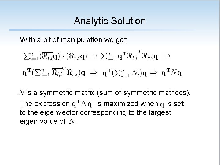
Analytic Solution With a bit of manipulation we get: is a symmetric matrix (sum of symmetric matrices). The expression is maximized when is set to the eigenvector corresponding to the largest eigen-value of.

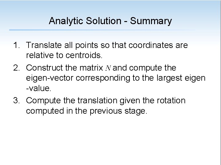
Analytic Solution - Summary 1. Translate all points so that coordinates are relative to centroids. 2. Construct the matrix and compute the eigen-vector corresponding to the largest eigen -value. 3. Compute the translation given the rotation computed in the previous stage.

In MATLAB (quaternion based approach) [01] [02] [03] [04] [05] [06] [07] [08] [09] [10] [11] [12] [13] [14] [15] [16] [17] [18] [19] function [T] = absolute. Orientation(points. In. Left, points. In. Right) mean. Left = mean(points. In. Left')'; mean. Right = mean(points. In. Right')'; M = points. In. Left*points. In. Right'; M = M - size(points. In. Left, 2)*mean. Left*mean. Right'; delta = [M(2, 3) - M(3, 2); M(3, 1) - M(1, 3); M(1, 2) - M(2, 1)]; N = [trace(M) delta'; delta (M+M'-trace(M)*eye(3))]; [eigen. Vectors, eigen. Values] = eig(N); [dummy, index] = max(diag(eigen. Values)); rotation = quaternion. To. Matrix(eigen. Vectors(: , index)); translation = mean. Right - rotation*mean. Left; T = [rotation, translation; [0, 0, 0, 1]];

In Python (matrix based approach) [01] def absolute_orientation(points_in_left, points_in_right): [02] import numpy as np [03] [04] num_points = len(points_in_left) [05] dim_points = len(points_in_left[0]) [06] [07] left_mat = np. array(points_in_left). T [08] right_mat = np. array(points_in_right). T [09] [10] left_mean = left_mat. mean(1) [11] right_mean = right_mat. mean(1) [12] left_M = left_mat - np. tile(left_mean, (num_points, 1)). T [13] right_M = right_mat - np. tile(right_mean, (num_points, 1)). T [14] [15] M = left_M. dot(right_M. T) [16] U, S, Vt = np. linalg. svd(M) [17] V=Vt. T [18] R = V. dot(np. diag((1, 1, np. linalg. det(U. dot(V))))). dot(U. T) [19] t = right_mean - R. dot(left_mean) [20] return R, t

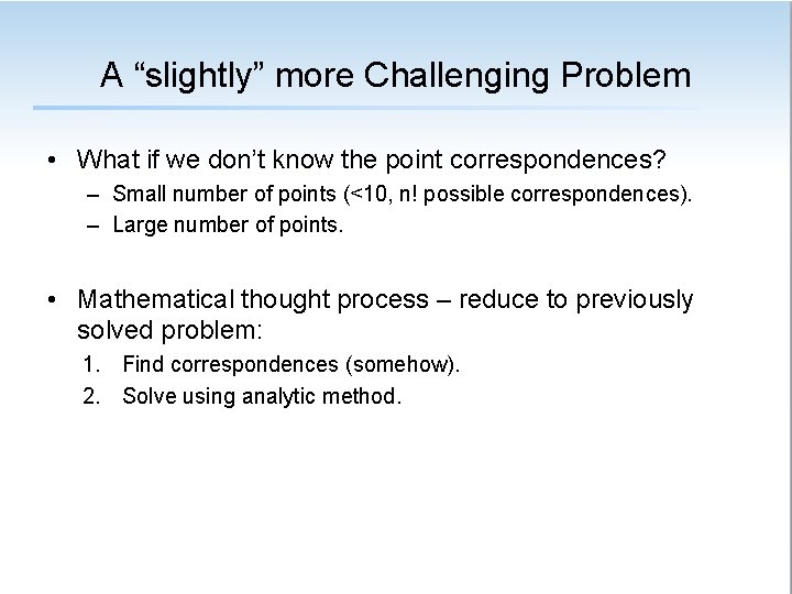
A “slightly” more Challenging Problem • What if we don’t know the point correspondences? – Small number of points (<10, n! possible correspondences). – Large number of points. • Mathematical thought process – reduce to previously solved problem: 1. Find correspondences (somehow). 2. Solve using analytic method.

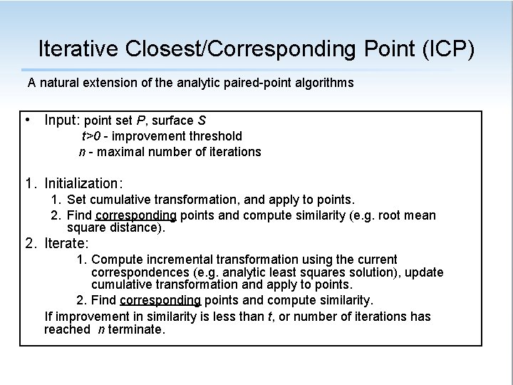
Iterative Closest/Corresponding Point (ICP) A natural extension of the analytic paired-point algorithms • Input: point set P, surface S t>0 - improvement threshold n - maximal number of iterations 1. Initialization: 1. Set cumulative transformation, and apply to points. 2. Find corresponding points and compute similarity (e. g. root mean square distance). 2. Iterate: 1. Compute incremental transformation using the current correspondences (e. g. analytic least squares solution), update cumulative transformation and apply to points. 2. Find corresponding points and compute similarity. If improvement in similarity is less than t, or number of iterations has reached n terminate.

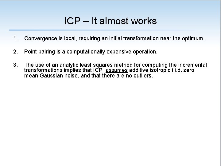
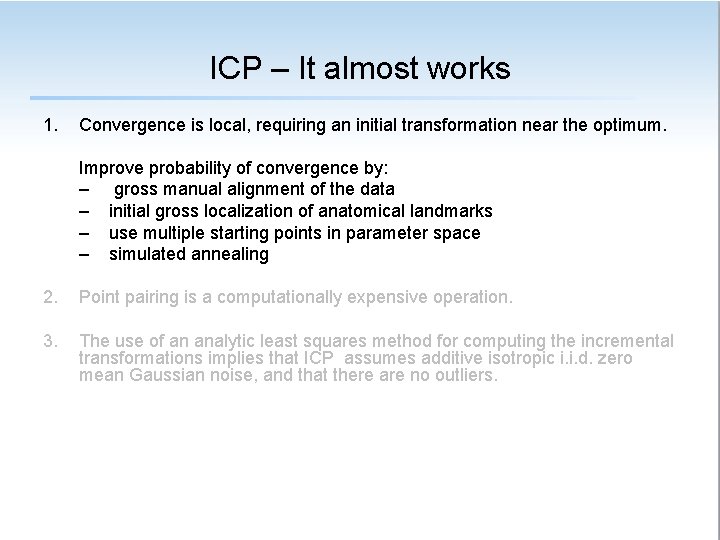
ICP – It almost works 1. Convergence is local, requiring an initial transformation near the optimum. 2. Point pairing is a computationally expensive operation. 3. The use of an analytic least squares method for computing the incremental transformations implies that ICP assumes additive isotropic i. i. d. zero mean Gaussian noise, and that there are no outliers.

ICP – It almost works 1. Convergence is local, requiring an initial transformation near the optimum. Improve probability of convergence by: – gross manual alignment of the data – initial gross localization of anatomical landmarks – use multiple starting points in parameter space – simulated annealing 2. Point pairing is a computationally expensive operation. 3. The use of an analytic least squares method for computing the incremental transformations implies that ICP assumes additive isotropic i. i. d. zero mean Gaussian noise, and that there are no outliers.

ICP – It almost works 1. Convergence is local, requiring an initial transformation near the optimum. 2. Point pairing is a computationally expensive operation. Accelerate run time by: – k. D tree spatial data structure – Cache closest points – Approximate nearest neighbor searching – Parallel nearest neighbor searching – Hierarchical data sampling 3. The use of an analytic least squares method for computing the incremental transformations implies that ICP assumes additive isotropic i. i. d. zero mean Gaussian noise, and that there are no outliers.

ICP – It almost works 1. Convergence is local, requiring an initial transformation near the optimum. 2. Point pairing is a computationally expensive operation. 3. The use of an analytic least squares method for computing the incremental transformations implies that ICP assumes additive isotropic i. i. d. zero mean Gaussian noise, and that there are no outliers. Replace analytic least squares methods with: – M-estimators – Least median of squares – Weighted least squares – Least trimmed squares – Use a fraction of the data

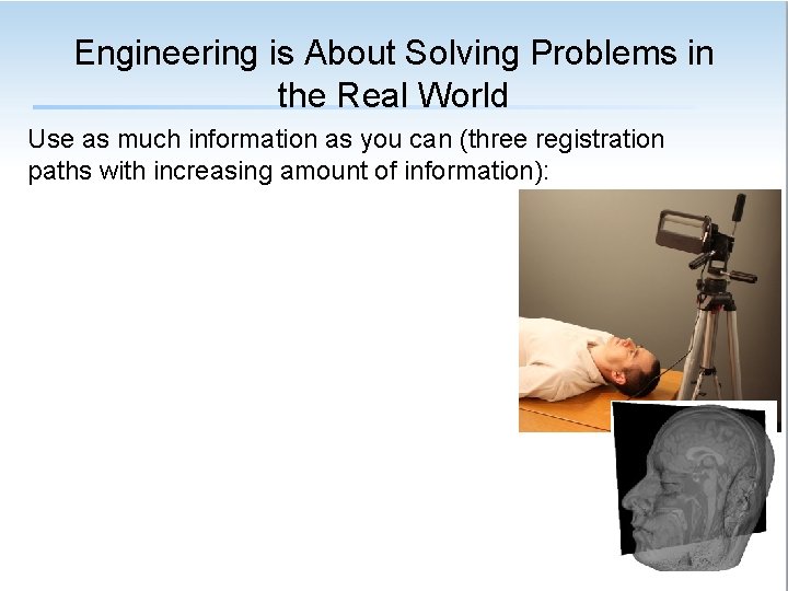
Engineering is About Solving Problems in the Real World Use as much information as you can (three registration paths with increasing amount of information):

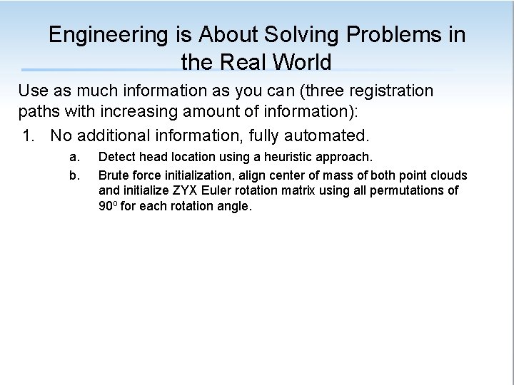
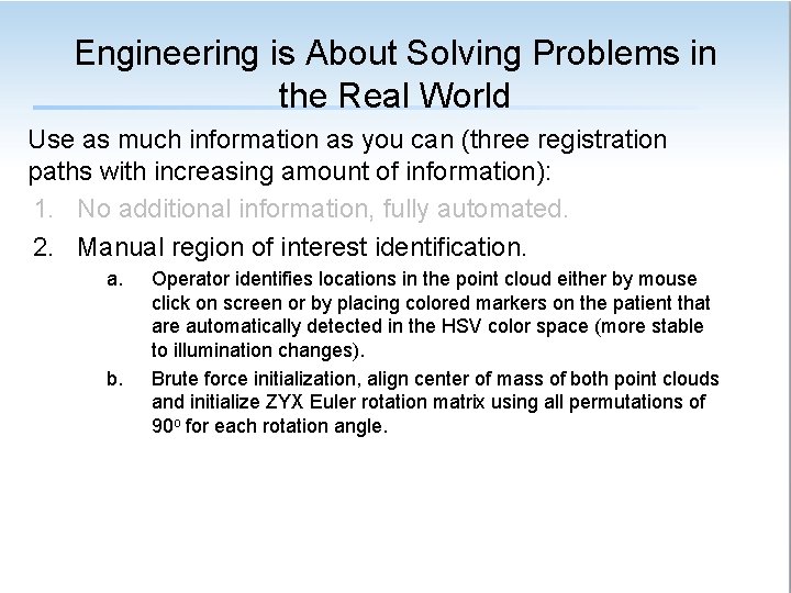
Engineering is About Solving Problems in the Real World Use as much information as you can (three registration paths with increasing amount of information): 1. No additional information, fully automated. a. b. Detect head location using a heuristic approach. Brute force initialization, align center of mass of both point clouds and initialize ZYX Euler rotation matrix using all permutations of 90 o for each rotation angle.

Engineering is About Solving Problems in the Real World Use as much information as you can (three registration paths with increasing amount of information): 1. No additional information, fully automated. 2. Manual region of interest identification. a. b. Operator identifies locations in the point cloud either by mouse click on screen or by placing colored markers on the patient that are automatically detected in the HSV color space (more stable to illumination changes). Brute force initialization, align center of mass of both point clouds and initialize ZYX Euler rotation matrix using all permutations of 90 o for each rotation angle.

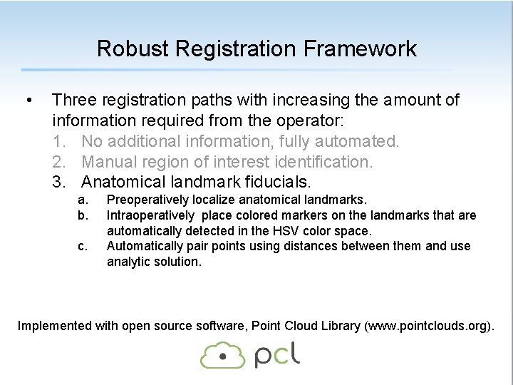
Robust Registration Framework • Three registration paths with increasing the amount of information required from the operator: 1. No additional information, fully automated. 2. Manual region of interest identification. 3. Anatomical landmark fiducials. a. b. c. Preoperatively localize anatomical landmarks. Intraoperatively place colored markers on the landmarks that are automatically detected in the HSV color space. Automatically pair points using distances between them and use analytic solution. Implemented with open source software, Point Cloud Library (www. pointclouds. org).

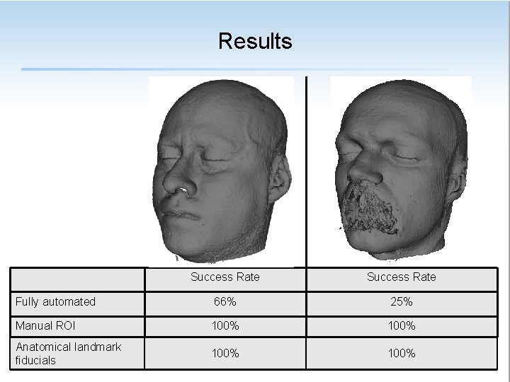
Results Success Rate Fully automated 66% 25% Manual ROI 100% Anatomical landmark fiducials 100%

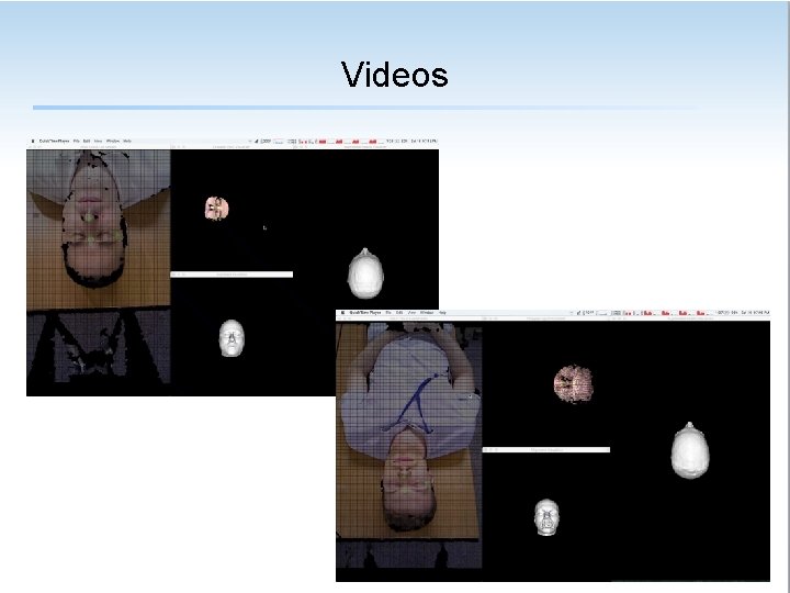
Videos

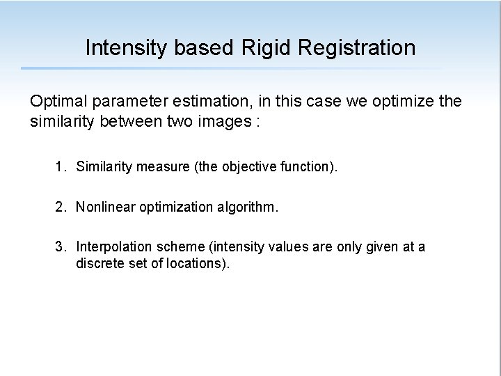
Intensity based Rigid Registration Optimal parameter estimation, in this case we optimize the similarity between two images : 1. Similarity measure (the objective function). 2. Nonlinear optimization algorithm. 3. Interpolation scheme (intensity values are only given at a discrete set of locations).

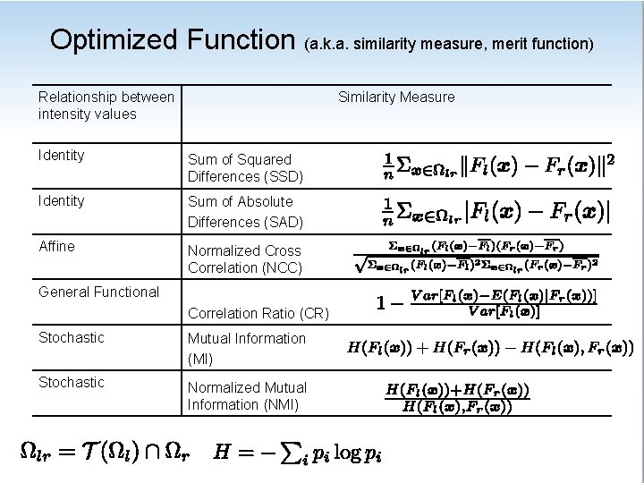
Optimized Function (a. k. a. similarity measure, merit function) Relationship between intensity values Similarity Measure Identity Sum of Squared Differences (SSD) Identity Sum of Absolute Differences (SAD) Affine Normalized Cross Correlation (NCC) General Functional Correlation Ratio (CR) Stochastic Mutual Information (MI) Stochastic Normalized Mutual Information (NMI)

Which Similarity Measure • • Computational complexity. Robustness. Capture range. Accuracy

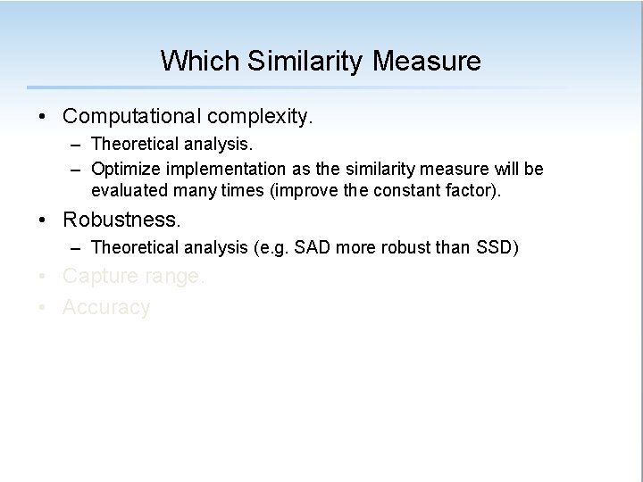
Which Similarity Measure • Computational complexity. – Theoretical analysis. – Optimize implementation as the similarity measure will be evaluated many times (improve the constant factor). • Robustness. – Theoretical analysis (e. g. SAD more robust than SSD) • Capture range. • Accuracy

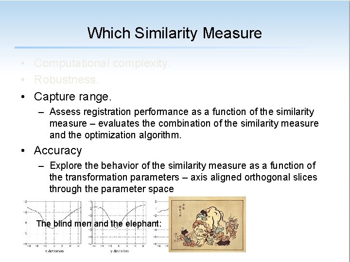
Which Similarity Measure • Computational complexity. • Robustness. • Capture range. – Assess registration performance as a function of the similarity measure – evaluates the combination of the similarity measure and the optimization algorithm. • Accuracy – Explore the behavior of the similarity measure as a function of the transformation parameters – axis aligned orthogonal slices through the parameter space The blind men and the elephant:

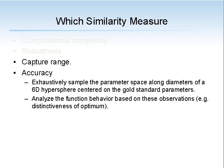
Which Similarity Measure • • Computational complexity. Robustness. Capture range. Accuracy – Exhaustively sample the parameter space along diameters of a 6 D hypersphere centered on the gold standard parameters. – Analyze the function behavior based on these observations (e. g. distinctiveness of optimum).

Optimization • General purpose optimization methods. • No single algorithm is optimal for all similarity measures (no-free-lunch theorem). • Initialize: – – Manual initialization via visual inspection. Automatic alignment to center of volume. Automatic alignment based on image moments. Paired-Point initialization. • Improve convergence range using heuristic search algorithms (e. g. simulated annealing) – double edged sword. Sometimes the desired pose is a local optimum and not a global one.

Interpolation • Linear interpolation – a compromise between accuracy and computational complexity. • May have adverse effects on the similarity measure. • B-spline interpolation - best tradeoff between accuracy and computational complexity, but we still use linear.

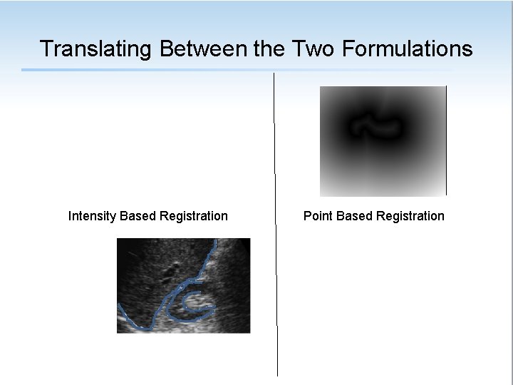
Translating Between the Two Formulations Intensity Based Registration Point Based Registration

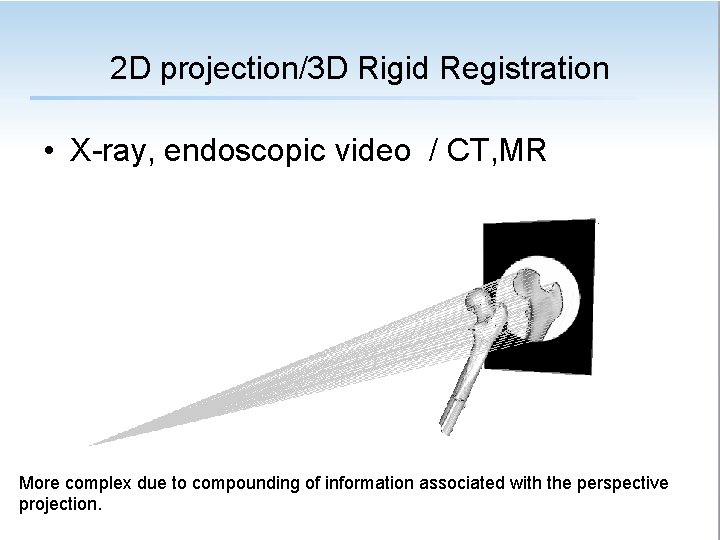
2 D projection/3 D Rigid Registration • X-ray, endoscopic video / CT, MR More complex due to compounding of information associated with the perspective projection.

Theory To Practice • In the past we spent significant efforts implementing known algorithms or used proprietary software. • Since the beginning of this century open source toolkits and applications that provide core functionalities have become ubiquitous. The Main Challenges: Maintenance and Sustainability

Insight Segmentation and Registration Toolkit (ITK) • ITK is a widely used image analysis toolkit. • Developed and maintained through support of the NLM (Terry S. Yoo, Michael J. Ackerman).

Insight Segmentation and Registration Toolkit (ITK) • Toolkit originally developed for analysis of medical images, as part of the Visible Human Project. • Foundation for [http: //www. itk. org/Wiki/ITK/Third_Party_Applications#Frameworks] – Toolkits: MITK, IGSTK, elastix, BRAINSFit, ANTS, orfeo… – Applications: 3 DSlicer, ITK-SNAP, med. INRIA… • Characteristics: – Flexibility through the use of C++ templates. – n. D images and algorithms. – filter pipeline architecture. C++ and Veteran non C++developers developer

itk. org/Wiki/Simple. ITK Lead developer: Bradley Lowekamp Contributors: Richard Beare Daniel Blezek David Chen David Cole David Doria Jean-Christophe Fillion-Robin Arnaud Gelas Ali Ghayoor Gabe Hart Luis Ibanez Hans Johnson Brad King Kasper Marstal Matt Mc. Cormick Dan Mueller Cory Quammen Kent Williams Ziv Yaniv

Simple. ITK • Favor usage simplicity over full flexibility: – Non templated C++ – 2 D/3 D and optionally 4 D image. – Standard, non-pipeline, architecture. • Subset of ITK functionality (300+ functional components, from basics , Add. Image. Filter, to advanced Image. Registration. Method). 1. Available for Python, R, C#, Java, Lua, Ruby, Tcl. 2. Binary Distributions for Many Platforms

Jupyter not Jupiter Notebooks From project’s site: “A web application that allows you to create and share documents that contain live code, equations, visualizations and explanatory text. ” Facilitates literate programming (concept introduced by D. Knuth): single document contains runnable code, natural language (e. g. algorithm description) and mathematical formulas. Increases the probability for reproducible research. Open Source

Simple. ITK Starter • Installation – https: //itk. org/Wiki/Simple. ITK • Learning – https: //github. com/Insight. Software. Consortium/Simple. ITK-Notebooks