RFAccelerating Structure Cooling Circuit Modeling Riku Raatikainen 16

RF-Accelerating Structure: Cooling Circuit Modeling Riku Raatikainen 16. 8. 2010

Content Part I Improved cooling circuit modeling - About me and my work at CERN - Introduction to improved cooling circuit modeling - Coupled thermal-structural modeling - Used engineering data - Improved cooling circuit model - Results for the SAS solved earlier by using CFD (computational fluid dynamics) - Conclusion Part II Case study: Test Lab Module - Introduction - Results - Conclusion Cooling Circuit Modeling, Riku Raatikainen, 16. 8. 2010

General • Summer trainee of HIP (3 months) • Student in Master’s Degree Programme of Mechanical Engineering majoring in Applied Mechanics • Main task and motivation - Improved cooling circuit modeling for TMM accelerating structures - The aim was to gain more efficient modeling method in order to solve current and future coupled thermal-structural models. Cooling Circuit Modeling, Riku Raatikainen, 16. 8. 2010

Introduction to improved cooling circuit modeling • Coupling CFD and structural analysis problems usually leads to complicated and computationally quite heavy models • This is due to coupling of the equations of continuum mechanics and fluid dynamics which especially in 3 D cases occur to be very complex • The improved cooling modeling that is to be presented here reduces this 3 D fluid flow into 1 D flow which is still capable of acting in a 3 D environment Cooling Circuit Modeling, Riku Raatikainen, 16. 8. 2010

Methodology Implementation to SAS cooling and comparing the efficiency to the model done by using 3 D CFD First test models Process Applying the method to up- to- date model Cooling Circuit Modeling, Riku Raatikainen, 16. 8. 2010

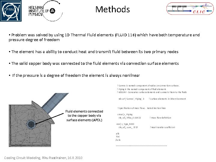
Methods • Problem was solved by using 1 D Thermal Fluid elements (FLUID 116) which have both temperature and pressure degree of freedom • The element has a ability to conduct heat and transmit fluid between its two primary nodes • The solid copper body was connected to the fluid elements via convection surface elements • If the pressure is a degree of freedom the element is always nonlinear ! Convec is named component of nodes on convection surfaces. ! Piping is the named component of fluid elements ! NDSURF - Generates surface elements and connects them to the fluids ndsur f, 'Convec', 'Piping', 3 ! Surface elements in 3 D environment ! Specification of mass flows - Note direction lines Fluid elements connected cmsel, s, Piping to the copper body via sfe, all, , hflux, , 0. 01922 ! Mass flow definition surface elements (APDL) esel, s, type, , 5000 sfe, all, , conv, , 3737 ! Heat transfer coefficient Cooling Circuit Modeling, Riku Raatikainen, 16. 8. 2010 alls fini /solu **********************

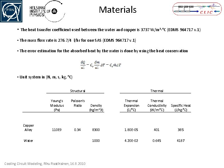
Materials • The heat transfer coefficient used between the water and copper is 3737 W/m²·°C (EDMS 964717 v. 1) • The mass flow rate is 276. 7/4 l/hr for one SAS (EDMS 964717 v. 1) • The error estimation for the absorbed heat by the water is done by using the heat conservation • Unit system in (N, m, s, kg, °C) Copper Alloy Structural Young's Modulus (Pa) Poisson's Ratio 110 E 9 0. 34 Water Cooling Circuit Modeling, Riku Raatikainen, 16. 8. 2010 Thermal Density (kg/m^3) Thermal Expansion (1/°C) Thermal Conductivity (W/m·°C) Specific Heat (J/kg·°C) 8300 1. 80 E-05 401 385 1000 4. 20 E-02 0. 645 4187

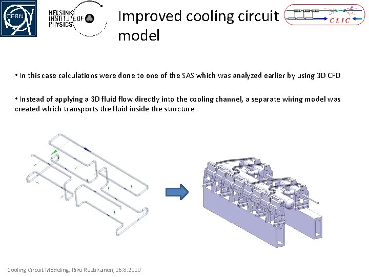
Improved cooling circuit model • In this case calculations were done to one of the SAS which was analyzed earlier by using 3 D CFD • Instead of applying a 3 D fluid flow directly into the cooling channel, a separate wiring model was created which transports the fluid inside the structure Cooling Circuit Modeling, Riku Raatikainen, 16. 8. 2010

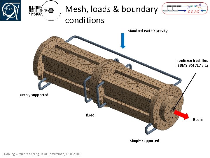
Mesh, loads & boundary conditions standard earth’s gravity nonlinear heat flux (EDMS 964717 v. 1) simply supported fixed Beam simply supported Cooling Circuit Modeling, Riku Raatikainen, 16. 8. 2010

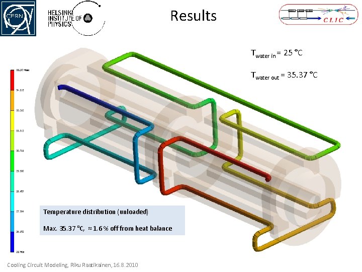
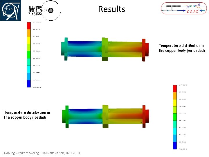
Results Twater in = 25 °C Twater out = 35. 37 °C Temperature distribution (unloaded) Max. 35. 37 °C, ≈ 1. 6 % off from heat balance Cooling Circuit Modeling, Riku Raatikainen, 16. 8. 2010

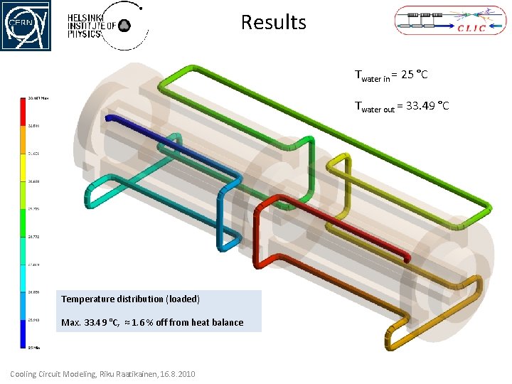
Results Twater in = 25 °C Twater out = 33. 49 °C Temperature distribution (loaded) Max. 33. 49 °C, ≈ 1. 6 % off from heat balance Cooling Circuit Modeling, Riku Raatikainen, 16. 8. 2010

Results Temperature distribution in the copper body (unloaded) Temperature distribution in the copper body (loaded) Cooling Circuit Modeling, Riku Raatikainen, 16. 8. 2010

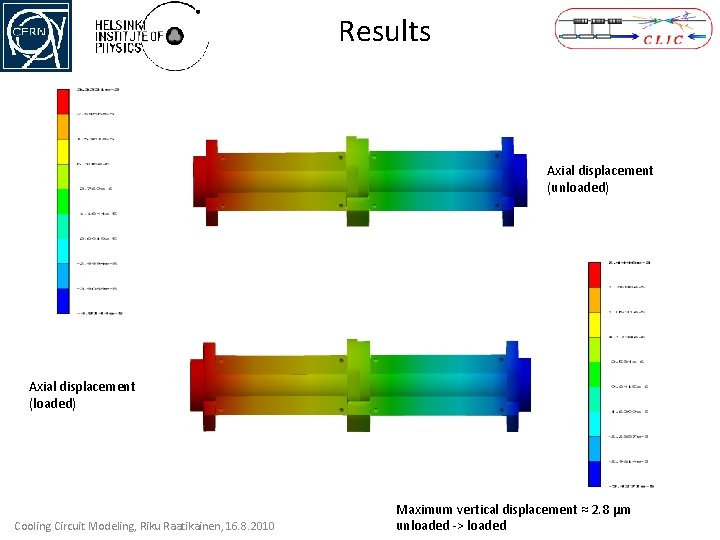
Results Axial displacement (unloaded) Axial displacement (loaded) Cooling Circuit Modeling, Riku Raatikainen, 16. 8. 2010 Maximum vertical displacement ≈ 2. 8 μm unloaded -> loaded

Conclusions • 1 D thermal fluid elements gives excellent results and they are in agreement with the previous ones • Computational time collapsed to only a fractions compared to the results obtained by using 3 D-CFD • New and more efficient method of solving coupled thermal-structural problems was achieved. • Moreover, the method provides an efficient tool to design optimisation Cooling Circuit Modeling, Riku Raatikainen, 16. 8. 2010

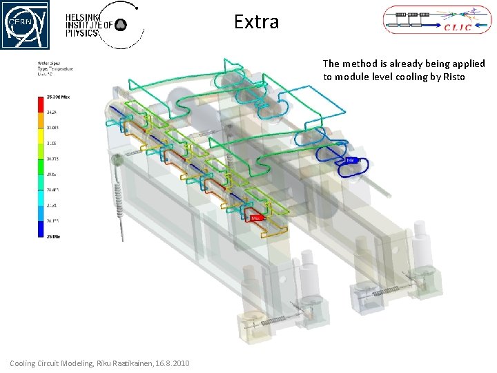
Extra The method is already being applied to module level cooling by Risto Cooling Circuit Modeling, Riku Raatikainen, 16. 8. 2010

Case Study Lab Test Module Cooling Circuit Modeling, Riku Raatikainen, 16. 8. 2010

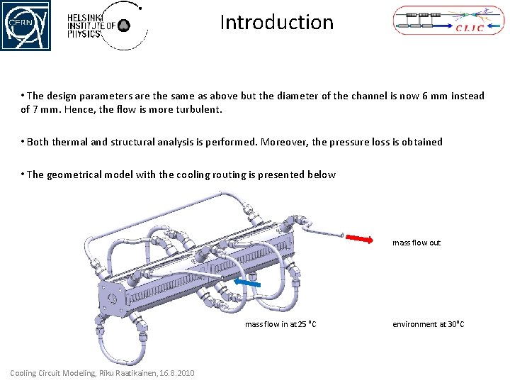
Introduction • The design parameters are the same as above but the diameter of the channel is now 6 mm instead of 7 mm. Hence, the flow is more turbulent. • Both thermal and structural analysis is performed. Moreover, the pressure loss is obtained • The geometrical model with the cooling routing is presented below mass flow out mass flow in at 25 °C Cooling Circuit Modeling, Riku Raatikainen, 16. 8. 2010 environment at 30°C

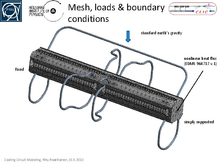
Mesh, loads & boundary conditions standard earth’s gravity nonlinear heat flux (EDMS 964717 v. 1) fixed simply supported Cooling Circuit Modeling, Riku Raatikainen, 16. 8. 2010

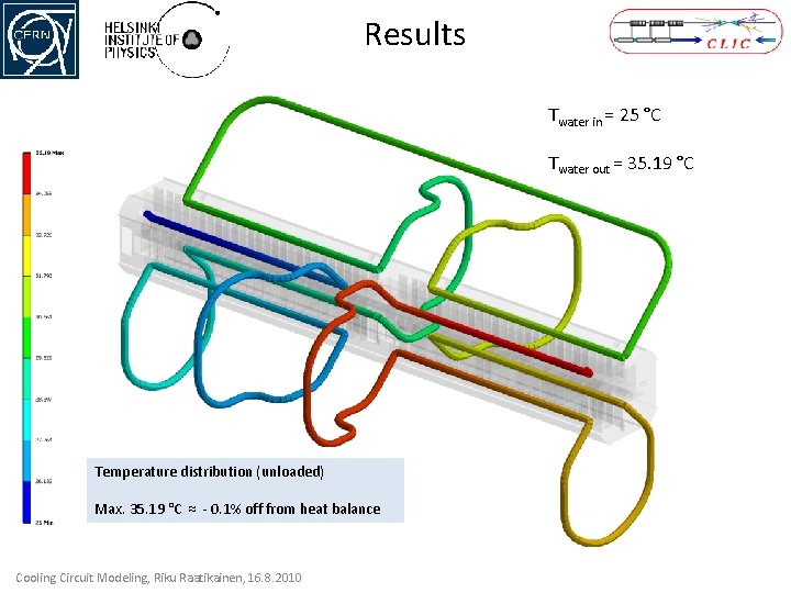
Results Twater in = 25 °C Twater out = 35. 19 °C Temperature distribution (unloaded) Max. 35. 19 °C ≈ - 0. 1% off from heat balance Cooling Circuit Modeling, Riku Raatikainen, 16. 8. 2010

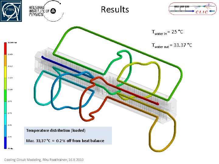
Results Twater in = 25 °C Twater out = 33. 37 °C Temperature distribution (loaded) Max. 33, 37 °C ≈ 0. 2 % off from heat balance Cooling Circuit Modeling, Riku Raatikainen, 16. 8. 2010

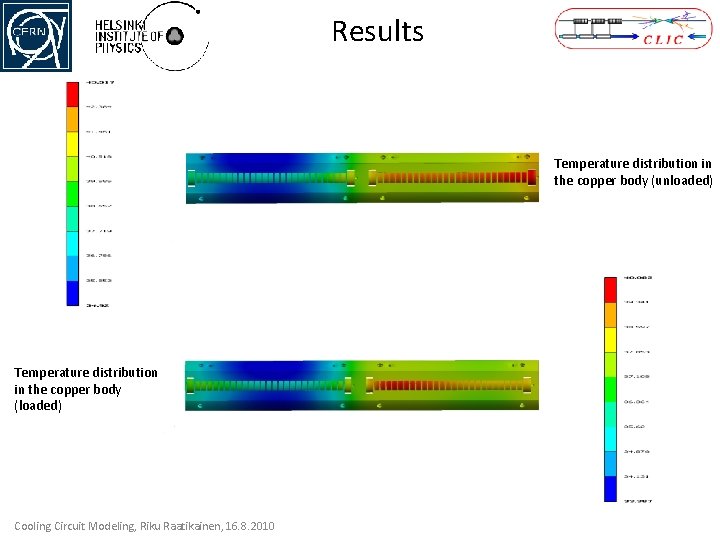
Results Temperature distribution in the copper body (unloaded) Temperature distribution in the copper body (loaded) Cooling Circuit Modeling, Riku Raatikainen, 16. 8. 2010

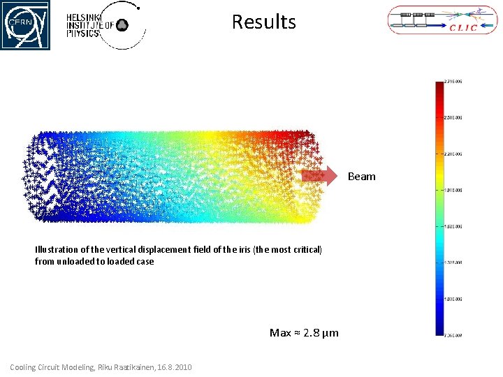
Results Beam Illustration of the vertical displacement field of the iris (the most critical) from unloaded to loaded case Max ≈ 2. 8 μm Cooling Circuit Modeling, Riku Raatikainen, 16. 8. 2010

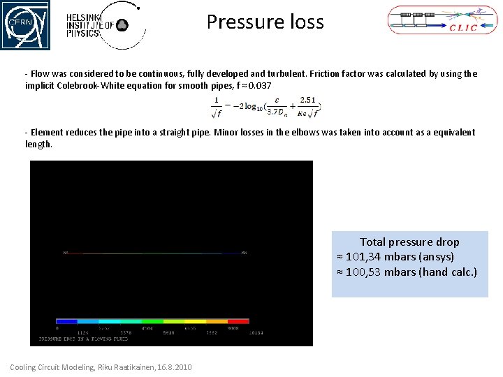
Pressure loss - Flow was considered to be continuous, fully developed and turbulent. Friction factor was calculated by using the implicit Colebrook-White equation for smooth pipes, f ≈ 0. 037 - Element reduces the pipe into a straight pipe. Minor losses in the elbows was taken into account as a equivalent length. Total pressure drop ≈ 101, 34 mbars (ansys) ≈ 100, 53 mbars (hand calc. ) Cooling Circuit Modeling, Riku Raatikainen, 16. 8. 2010

Conclusions • The 1 D fluid elements are capable of working efficiently also in more complex geometries • For more even thermal distribution, a smaller mass flow rate can be used for loaded case • Moreover, different kinds of support boundary conditions can be used to adjust the displacement field • Pressure loss can minimized by using larger radius tubes and bendings, if needed Cooling Circuit Modeling, Riku Raatikainen, 16. 8. 2010

Thank you