Revisiting Pipelined Parallelism in MultiJoin Query Processing Bin

Revisiting Pipelined Parallelism in Multi-Join Query Processing Bin Liu and Elke A. Rundensteiner Worcester Polytechnic Institute (binliu|rundenst)@cs. wpi. edu http: //www. davis. wpi. edu/dsrg VLDB 2005 1

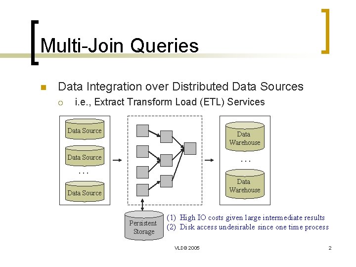
Multi-Join Queries n Data Integration over Distributed Data Sources ¡ i. e. , Extract Transform Load (ETL) Services Data Source Data Warehouse … Data Source … Data Warehouse Data Source Persistent Storage (1) High IO costs given large intermediate results (2) Disk access undesirable since one time process VLDB 2005 2

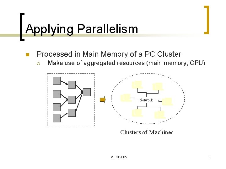
Applying Parallelism n Processed in Main Memory of a PC Cluster ¡ Make use of aggregated resources (main memory, CPU) Network Clusters of Machines VLDB 2005 3

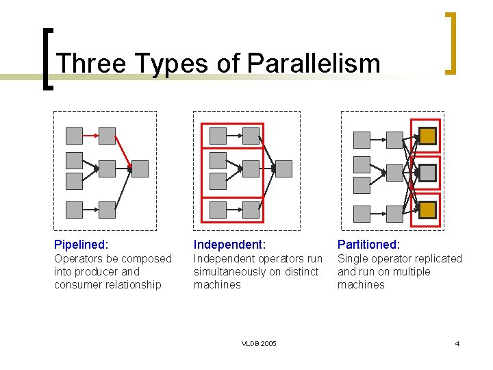
Three Types of Parallelism Pipelined: Independent: Partitioned: Operators be composed into producer and consumer relationship Independent operators run simultaneously on distinct machines Single operator replicated and run on multiple machines VLDB 2005 4

Basics of Hash Join Two-Phase Hash Join [SD 89, LTS 90] n Demonstrated High Performance Potential High Degree of Parallelism ¡ ¡ key ID Date … OID Item … 0011 5/13 … 0011 IPC … 0012 5/14 … 0012 HPS … … … … Orders value (2) Probe hash tables and output results (1) Build hash tables of Orders based on ID Line. Items OID Item … ID Date … 0011 IPC … 0011 5/13 … 0012 HPS … 0012 5/14 … … … … Line. Items VLDB 2005 Orders 5

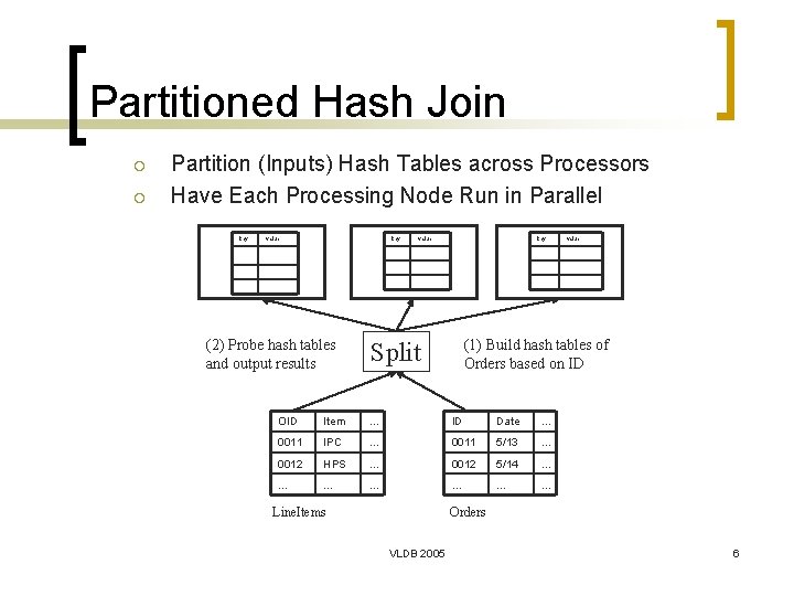
Partitioned Hash Join ¡ ¡ Partition (Inputs) Hash Tables across Processors Have Each Processing Node Run in Parallel key value (2) Probe hash tables and output results Split key (1) Build hash tables of Orders based on ID OID Item … ID Date … 0011 IPC … 0011 5/13 … 0012 HPS … 0012 5/14 … … … … Line. Items value Orders VLDB 2005 6

Left-Deep Tree [SD 90] Example Join Graph R 9 R 8 R 2 R 6 R 1 R 3 R 7 R 5 R 4 Left-Deep Query Tree B 8 P 8 (9) Scan R 9 – Probe P 8 – Output B 7 P 7 R 9 B 1 P 1 R 1 (3) Scan R 3 – Probe P 2 – Build B 3 R 2 (8) Scan R 8 – Probe P 7 – Build B 8 … R 8 B 2 P 2 Steps: (2) Scan R 2 – Probe P 1 – Build B 2 (1) Scan R 1 – Build R 1 VLDB 2005 7

Right-Deep Tree [SD 90] Example Join Graph R 9 R 8 R 2 R 6 R 1 R 3 R 7 R 5 R 4 Right-Deep Query Tree B 8 P 8 R 9 B 7 P 7 R 8 B 2 P 2 (1) (2) (3) (4) Scan R 2 – Build R 1, Scan R 3 – Build R 2, …, Scan R 9 – Build R 8 B 1 P 1 R 3 VLDB 2005 (2) Scan R 1, Probe P 2, …, Probe P 8 R 2 R 1 8

Tradeoffs Between Left and Right Trees n Right-Deep Good potential for pipelined parallelism. Intermediate results exist only as a stream. Size of building relations can be predicted accurately. Large memory consumption. n Left-Deep Less memory consumption Less pipelined parallelism VLDB 2005 9

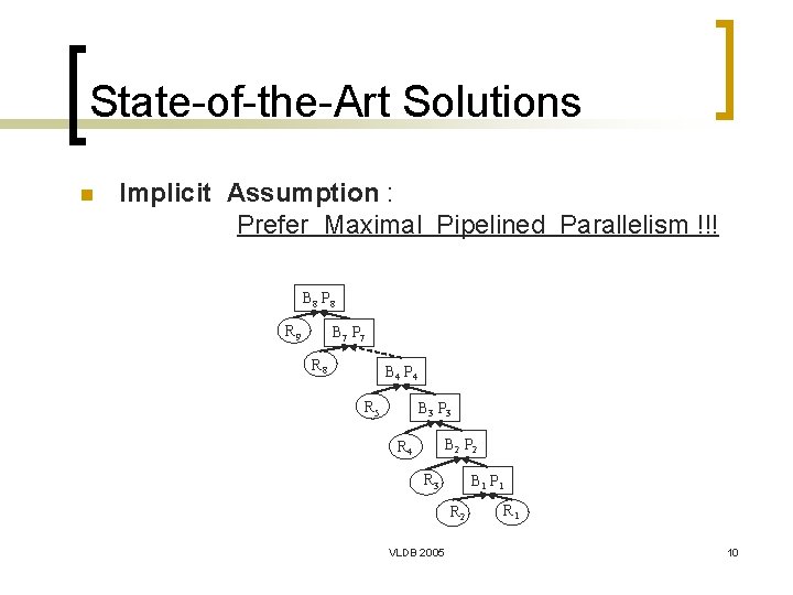
State-of-the-Art Solutions n Implicit Assumption : Prefer Maximal Pipelined Parallelism !!! B 8 P 8 R 9 B 7 P 7 R 8 B 4 P 4 R 5 B 3 P 3 B 2 P 2 R 4 R 3 B 1 P 1 R 2 VLDB 2005 R 1 10

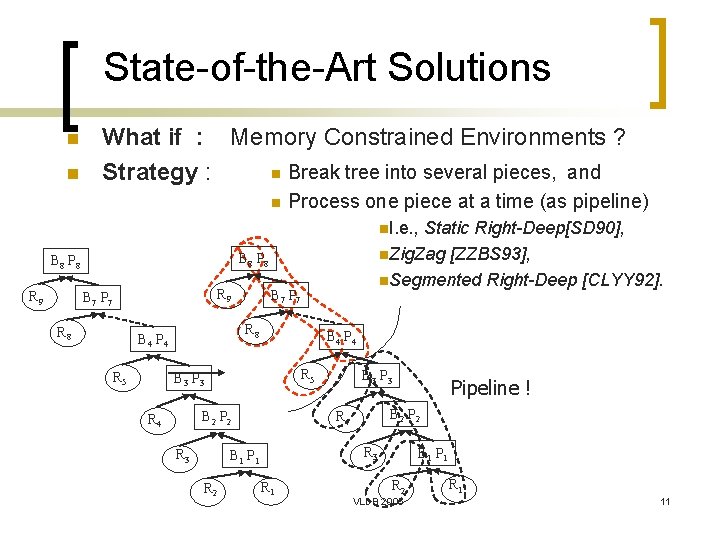
State-of-the-Art Solutions n n What if : Memory Constrained Environments ? n Break tree into several pieces, and Strategy : n Process one piece at a time (as pipeline) n. I. e. , B 8 P 8 R 9 Static Right-Deep[SD 90], n. Zig. Zag [ZZBS 93], n. Segmented Right-Deep [CLYY 92]. R 9 B 7 P 7 R 8 B 4 P 4 R 5 B 7 P 7 B 4 P 4 R 5 B 3 P 3 R 3 B 1 P 1 R 2 R 1 Pipeline ! B 2 P 2 R 4 B 3 P 3 B 1 P 1 R 2 VLDB 2005 R 1 11

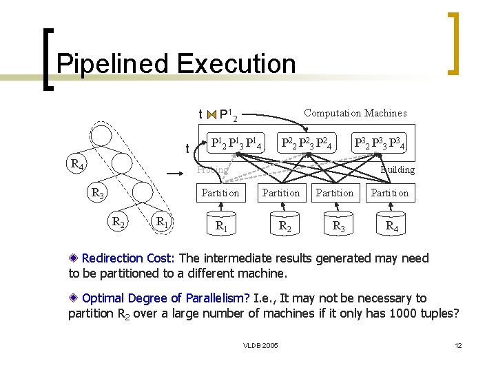
Pipelined Execution t t R 4 Computation Machines P 12 P 1 3 P 1 4 P 2 2 P 2 3 P 2 4 P 3 2 P 3 3 P 3 4 Probing R 3 Partition R 2 R 1 Building Partition R 1 R 2 Partition R 3 Partition R 4 Redirection Cost: The intermediate results generated may need to be partitioned to a different machine. Optimal Degree of Parallelism? I. e. , It may not be necessary to partition R 2 over a large number of machines if it only has 1000 tuples? VLDB 2005 12

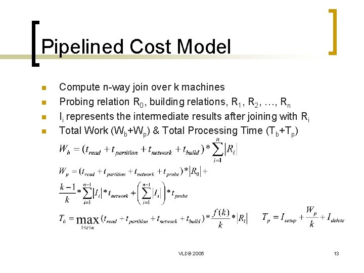
Pipelined Cost Model n n Compute n-way join over k machines Probing relation R 0, building relations, R 1, R 2, …, Rn Ii represents the intermediate results after joining with Ri Total Work (Wb+Wp) & Total Processing Time (Tb+Tp) VLDB 2005 13

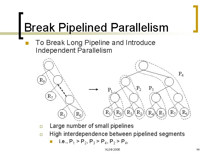
Break Pipelined Parallelism n To Break Long Pipeline and Introduce Independent Parallelism P 4 R 9 R 7 R 1 ¡ ¡ P 2 P 3 R 2 R 4 P 1 R 0 R 5 R 7 R 6 Large number of small pipelines High interdependence between pipelined segments n i. e. , P 1 > P 2, P 3 > P 4, P 2 > P 4, VLDB 2005 14

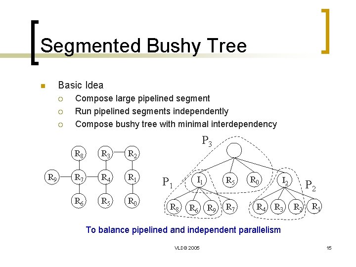
Segmented Bushy Tree Basic Idea n ¡ ¡ ¡ R 9 Compose large pipelined segment Run pipelined segments independently Compose bushy tree with minimal interdependency R 8 R 3 R 2 R 7 R 4 R 1 R 6 R 5 R 0 P 3 I 1 P 1 R 8 R 6 R 5 R 9 R 7 R 0 R 4 I 2 R 3 P 2 R 1 To balance pipelined and independent parallelism VLDB 2005 15

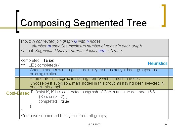
Composing Segmented Tree Input: A connected join graph G with n nodes. Number m specifies maximum number of nodes in each graph. Output: Segmented bushy tree with at least n/m subtrees. completed = false; Heuristics WHILE (!completed) { Choose node V with largest cardinality that has not yet been grouped as probing relation; Enumerate all subgraphs starting from V with at most m nodes; Choose best subgraph, mark nodes in this group as having been selected in original join graph; Cost-Based IF !(exist K, K is a connected subgraph of G with unselected nodes) && (K. size() >= 2) { completed = true; } } Compose segmented bushy tree from all groups; VLDB 2005 16

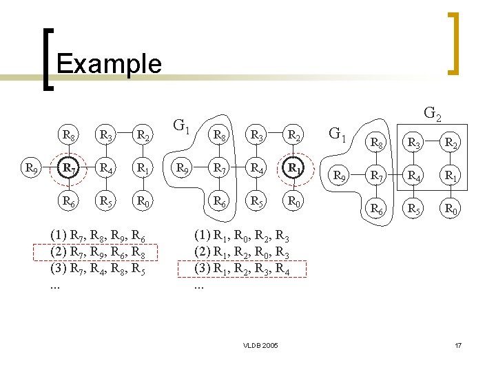
Example R 9 R 8 R 3 R 2 R 7 R 4 R 1 R 6 R 5 R 0 (1) R 7, R 8, R 9, R 6 (2) R 7, R 9, R 6, R 8 (3) R 7, R 4, R 8, R 5. . . G 1 R 9 R 8 R 3 R 2 R 7 R 4 R 1 R 6 R 5 R 0 G 2 G 1 R 8 R 3 R 2 R 9 R 7 R 4 R 1 R 6 R 5 R 0 (1) R 1, R 0, R 2, R 3 (2) R 1, R 2, R 0, R 3 (3) R 1, R 2, R 3, R 4. . . VLDB 2005 17

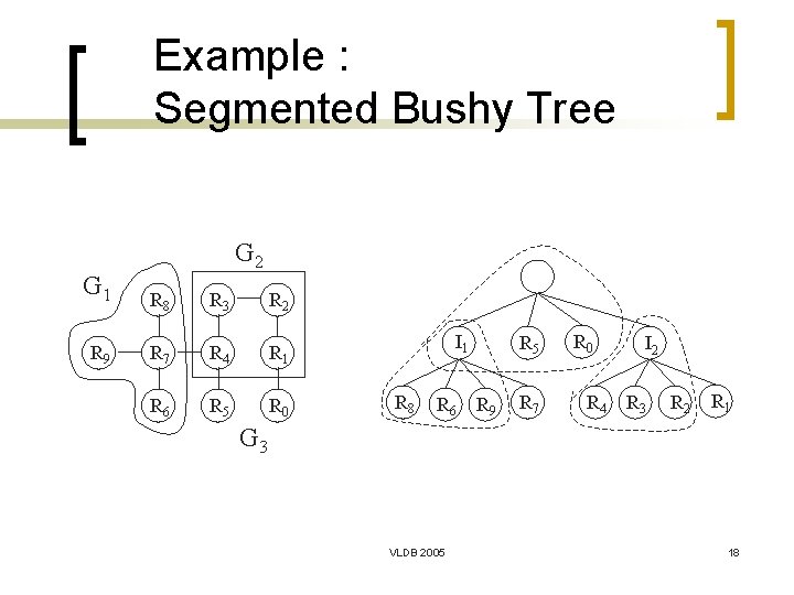
Example : Segmented Bushy Tree G 2 G 1 R 8 R 3 R 2 R 9 R 7 R 4 R 1 R 6 R 5 R 0 I 1 R 8 R 6 R 5 R 9 R 7 R 0 R 4 I 2 R 3 R 2 R 1 G 3 VLDB 2005 18

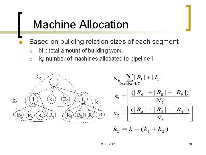
Machine Allocation n Based on building relation sizes of each segment Nb: total amount of building work. ki: number of machines allocated to pipeline i ¡ ¡ k 3 k 1 R 8 I 1 R 6 Nb = R 5 R 9 R 7 R 0 R 4 I 2 R 3 k 2 R 1 VLDB 2005 19

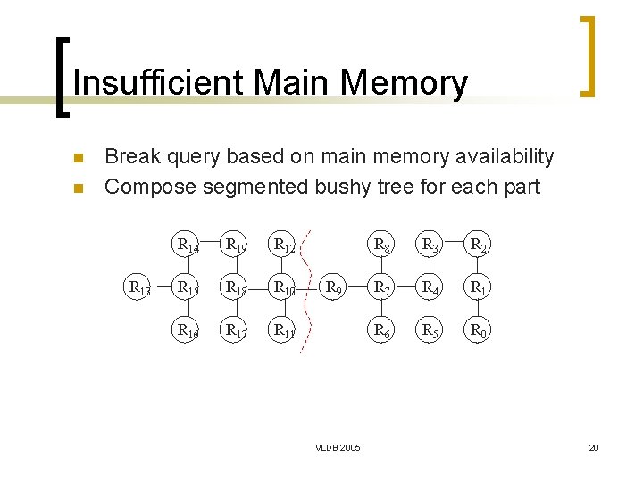
Insufficient Main Memory n n Break query based on main memory availability Compose segmented bushy tree for each part R 13 R 14 R 19 R 12 R 15 R 18 R 10 R 16 R 17 R 11 R 9 VLDB 2005 R 8 R 3 R 2 R 7 R 4 R 1 R 6 R 5 R 0 20

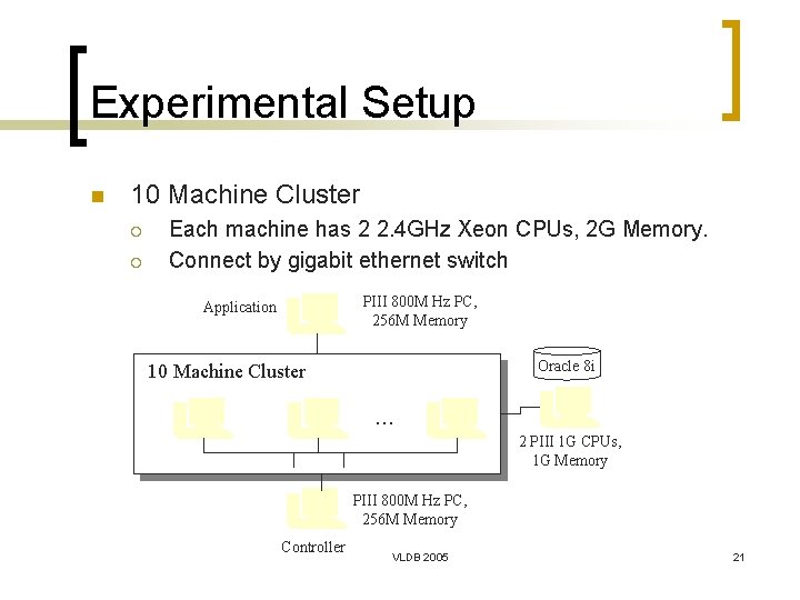
Experimental Setup n 10 Machine Cluster ¡ ¡ Each machine has 2 2. 4 GHz Xeon CPUs, 2 G Memory. Connect by gigabit ethernet switch PIII 800 M Hz PC, 256 M Memory Application Oracle 8 i 10 Machine Cluster . . . 2 PIII 1 G CPUs, 1 G Memory PIII 800 M Hz PC, 256 M Memory Controller VLDB 2005 21

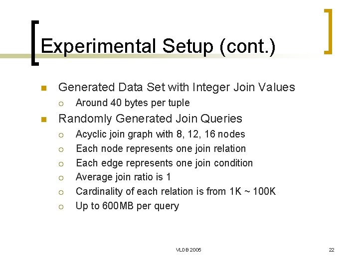
Experimental Setup (cont. ) n Generated Data Set with Integer Join Values ¡ n Around 40 bytes per tuple Randomly Generated Join Queries ¡ ¡ ¡ Acyclic join graph with 8, 12, 16 nodes Each node represents one join relation Each edge represents one join condition Average join ratio is 1 Cardinality of each relation is from 1 K ~ 100 K Up to 600 MB per query VLDB 2005 22

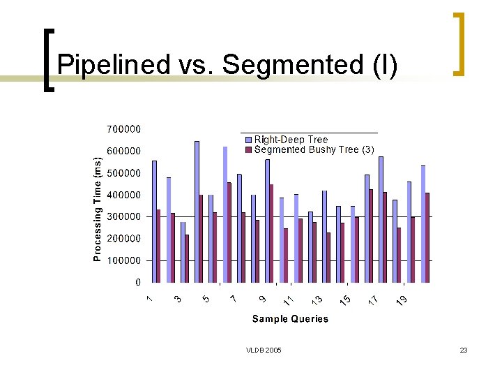
Pipelined vs. Segmented (I) VLDB 2005 23

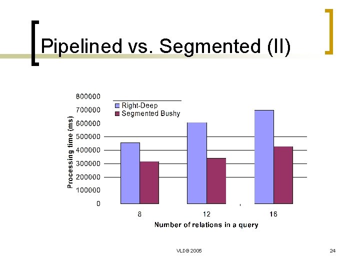
Pipelined vs. Segmented (II) VLDB 2005 24

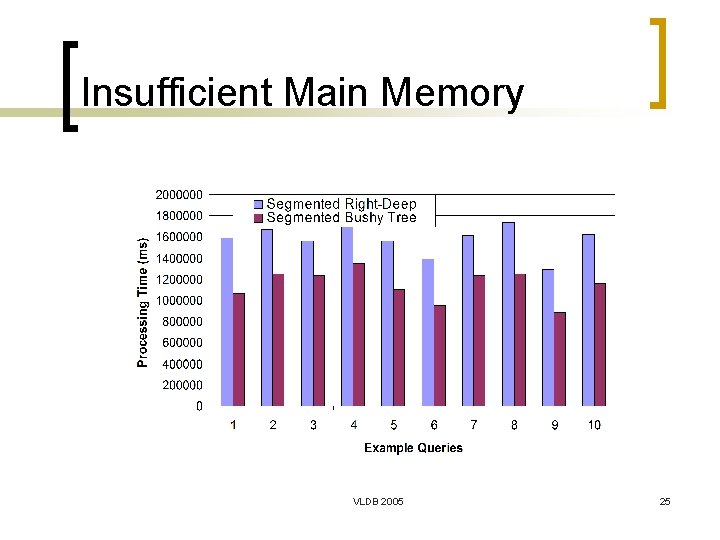
Insufficient Main Memory VLDB 2005 25

Related Work n n n n [SD 90] Tradeoffs in processing complex join queries via hashing in multiprocessor database machines. VLDB 1990. [CLYY 92] Using segmented right deep trees for execution of pipelined hash joins. VLDB 1992. [MLD 94] Parallel hash based join algorithms for a shared everything environment. TKDE 1994. [MD 97] Data placement in shared nothing parallel database systems. VLDB 1997. [WFA 95] Parallel evaluation of multi-join queries. SIGMOD 1995. [HCY 94] On parallel execution of multiple pipelined hash joins. SIGMOD 1994. [DNSS 92] Practical skew handling in parallel joins. VLDB 1992. [SHCF 03] Flux: an adaptive partitioning operator for continuous query systems. ICDE, 2003. VLDB 2005 26

Conclusions n Observation: Maximal pipelined hash join processing ¡ n Hypothesis: Worthwhile to incorporate independent parallelism into processing ¡ n Both, so several shorter pipelines in parallel Solution: Segmented bushy tree processing ¡ n Redirection costs? optimal degree of parallelism? Heuristics and cost-driven algorithm developed Validation : Extensive experimental studies ¡ Achieve around 50% improvement over pure pipelined VLDB 2005 processing 27