Review Session JehanFranois Pris Agenda Statistical Analysis of

Review Session Jehan-François Pâris

Agenda Statistical Analysis of Outputs n Operational Analysis n Case Studies n Linear Regression n

How to use this presentation n Most problems have ¨ One slide stating the problem ¨ One slide explaining how to solve the problem ¨ One slide allowing you to check your answer You will learn more by trying first to do the problems on your own than by reading their solutions n Do not forget either to review the problems in the original notes n

Statistical Analysis of Outputs

The big picture n The problems ¨ Constructing confidence intervals ¨ Handling auto correlated data n The tools ¨ Central-Limit Theorem ¨ Wilson’s formula ¨ Batch means (and regeneration) ¨ RNG tricks

Confidence Intervals n Distinguish between ¨ CIs for means n CSIM does it for you ¨ CIs for proportions n We are on our own n Major issue is independence of data points n CSIM uses batch means

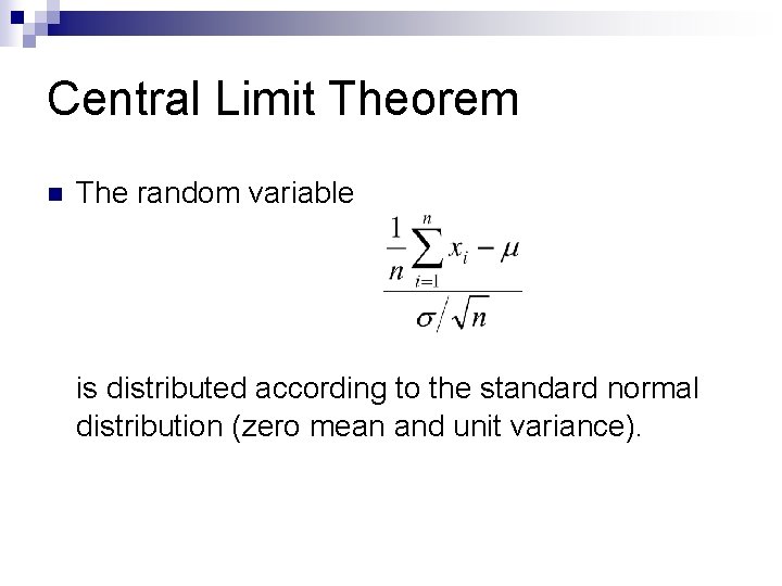
Central Limit Theorem n If the n mutually independent random variables x 1, x 2, …, xn have the same distribution, and if their mean m and their variance s 2 exist then …

Central Limit Theorem n The random variable is distributed according to the standard normal distribution (zero mean and unit variance).

CI for means (I) n For large values of n, the (1 - )% confidence interval for m is given by n with

CI for means (II) n F(z) is taken from a table of the normal distribution ¨ F(0. 025) n For smaller values of n, we have to use Student’s t random variable ¨ Wider n = 1. 96 CIs We replace s by the sample standard deviation s

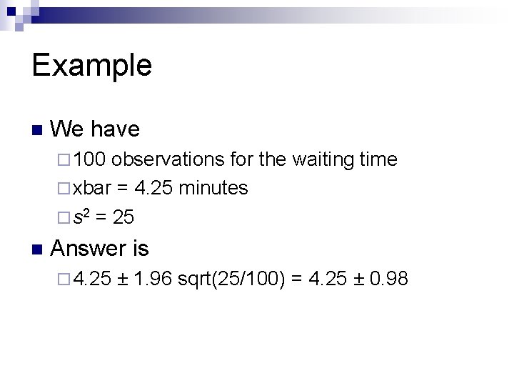
Example n We have ¨ 100 observations for the waiting time ¨ xbar = 4. 25 minutes ¨ s 2 = 25

Example n We have ¨ 100 observations for the waiting time ¨ xbar = 4. 25 minutes ¨ s 2 = 25 n Answer is ¨ 4. 25 ± 1. 96 sqrt(25/100) = 4. 25 ± 0. 98

CI for proportions n A proportion represents the probability P(X ) for some fixed threshold ¨ 97% of our customers have to wait less than one minute n Distributed according to a binomial law ¨ Use Wilson’s formula

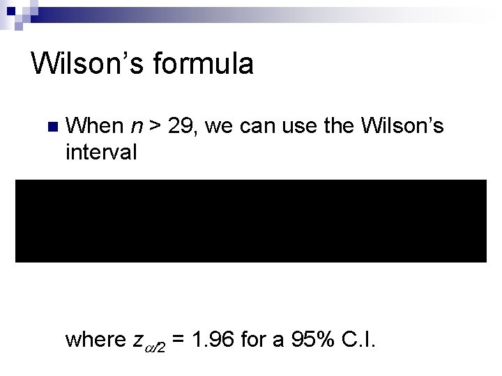
Wilson’s formula n When n > 29, we can use the Wilson’s interval where za/2 = 1. 96 for a 95% C. I.

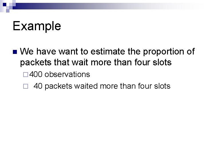
Example n We have want to estimate the proportion of packets that wait more than four slots ¨ 400 observations ¨ 40 packets waited more than four slots

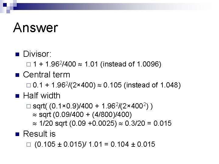
Answer n Divisor: ¨ 1 n + 1. 962/400 1. 01 (instead of 1. 0096) Central term ¨ 0. 1 n + 1. 962/(2× 400) 0. 105 (instead of 1. 048) Half width ¨ sqrt( (0. 1× 0. 9)/400 + 1. 962/(2× 4002) ) sqrt (0. 09/400 + (4/800)/400) 1/20 sqrt (0. 09 +0. 0025) 0. 3/20 = 0. 015 n Result is ¨ (0. 105 ± 0. 015)/ 1. 01 = 0. 104 ± 0. 015

Batch means (I) n Simulation data are often autocorrelated ¨ Packet delays in ALOHA ¨ Waiting times in queues ¨… n Batch means reduce (but do not completely eliminate) that effect

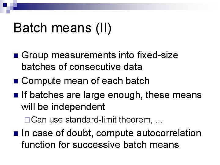
Batch means (II) Group measurements into fixed-size batches of consecutive data n Compute mean of each batch n If batches are large enough, these means will be independent n ¨ Can n use standard-limit theorem, … In case of doubt, compute autocorrelation function for successive batch means

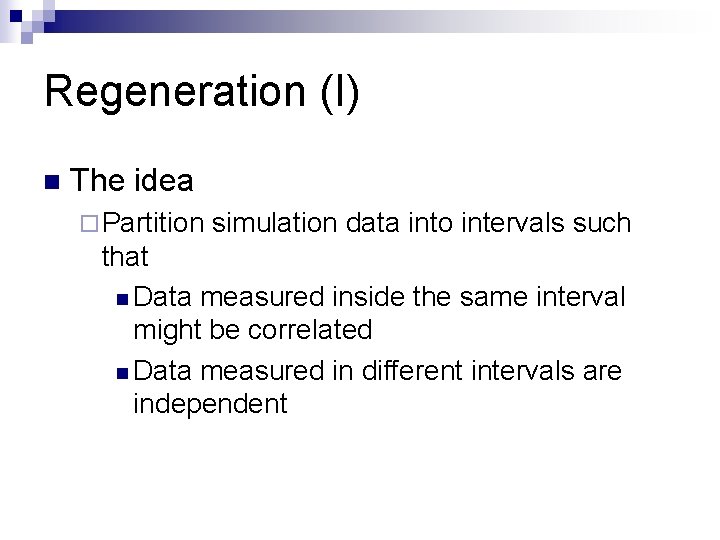
Regeneration (I) n The idea ¨ Partition simulation data into intervals such that n Data measured inside the same interval might be correlated n Data measured in different intervals are independent

Regeneration (II) n How? ¨ System goes to a regeneration point each time n Its queues become empty n All the disk drives are operational n… ¨ Criterion is system specific

Streams n When you want to evaluate two different configurations of a system, it is often good idea to use separate random number streams for arrivals and service times ¨ Arrival times remain unchanged when we change other parameters of the system

Operational Analysis

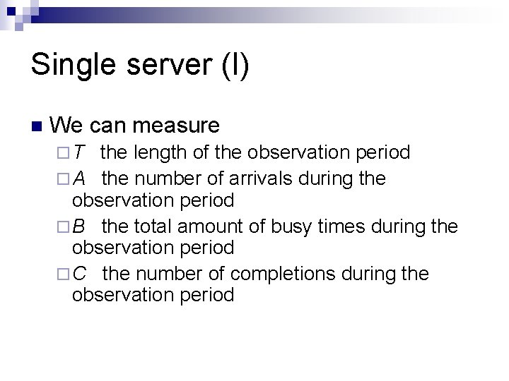
Single server (I) n We can measure ¨T the length of the observation period ¨ A the number of arrivals during the observation period ¨ B the total amount of busy times during the observation period ¨ C the number of completions during the observation period

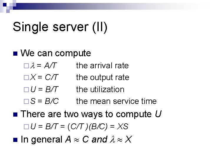
Single server (II) n We can compute ¨l = A/T ¨ X = C/T ¨ U = B/T ¨ S = B/C n There are two ways to compute U ¨U n the arrival rate the output rate the utilization the mean service time = B/T = (C/T )(B/C) = XS In general A C and l X

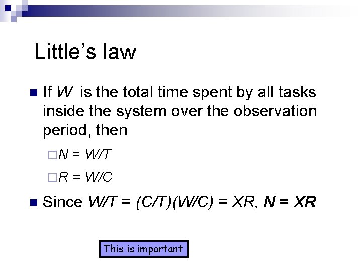
Little’s law n n If W is the total time spent by all tasks inside the system over the observation period, then ¨N = W/T ¨R = W/C Since W/T = (C/T)(W/C) = XR, N = XR This is important

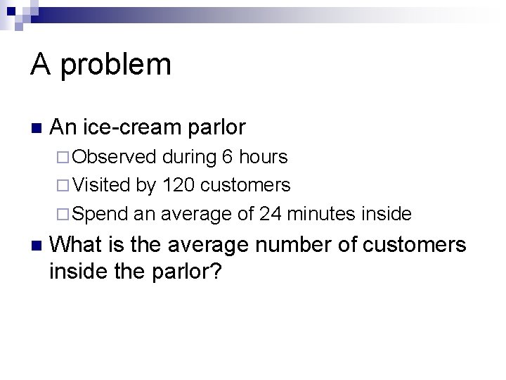
A problem n An ice-cream parlor ¨ Observed during 6 hours ¨ Visited by 120 customers ¨ Spend an average of 24 minutes inside n What is the average number of customers inside the parlor?

Answer n We compute X and apply Little’s Law

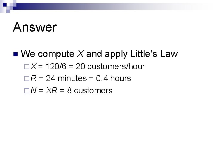
Answer n We compute X and apply Little’s Law ¨X = 120/6 = 20 customers/hour ¨ R = 24 minutes = 0. 4 hours ¨ N = XR = 8 customers

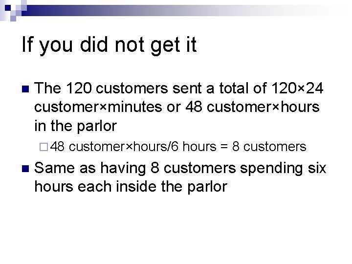
If you did not get it n The 120 customers sent a total of 120× 24 customer×minutes or 48 customer×hours in the parlor ¨ 48 n customer×hours/6 hours = 8 customers Same as having 8 customers spending six hours each inside the parlor

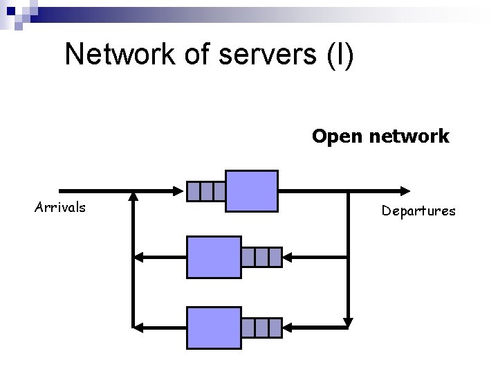
Network of servers (I) Open network Arrivals Departures

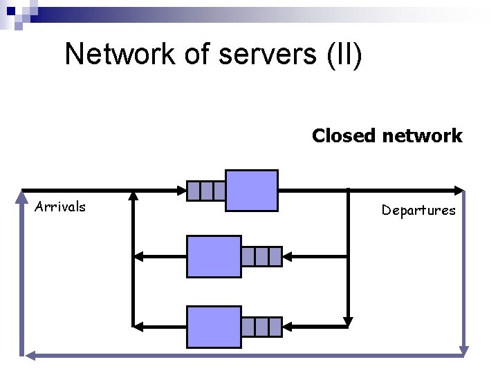
Network of servers (II) Closed network Arrivals Departures

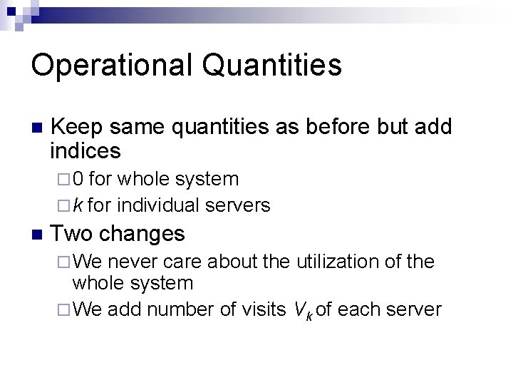
Operational Quantities n Keep same quantities as before but add indices ¨ 0 for whole system ¨ k for individual servers n Two changes ¨ We never care about the utilization of the whole system ¨ We add number of visits Vk of each server

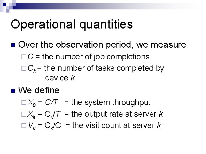
Operational quantities n Over the observation period, we measure ¨C = the number of job completions ¨ Ck = the number of tasks completed by device k n We define ¨ X 0 = C/T = the system throughput ¨ Xk = Ck/T = the output rate at server k ¨ Vk = Ck/C = the visit count at server k

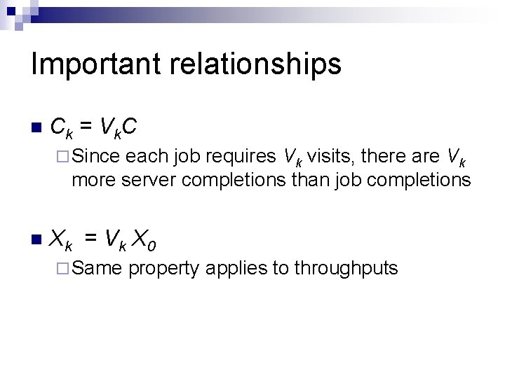
Important relationships n Ck = Vk. C ¨ Since each job requires Vk visits, there are Vk more server completions than job completions n Xk = Vk X 0 ¨ Same property applies to throughputs

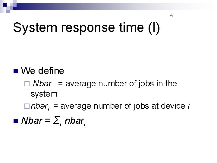
System response time (I) n We define Nbar = average number of jobs in the system ¨ nbari = average number of jobs at device i ¨ n Nbar = Σi nbari

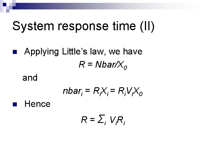
System response time (II) n n Applying Little’s law, we have R = Nbar/X 0 and nbari = Ri. Xi = Ri. Vi. X 0 Hence R = Σ i V i. R i

Note n This result is trivial ¨ The total time spent by a job in the system is the sum of the times spent at each server n This includes the time spent waiting in the server queues

Problem 1 n A job requires ¨ 100 ms of CPU time ¨ 9 disk accesses Each disk access takes 7 ms n We want n ¨ VCPU and SCPU

Answer n We now that jobs get CPU first and last ¨ VCPU n = 10 Then ¨ SCPU = 100/10 =10 s

Bottleneck analysis (I) A system has one CPU and one disk drive n It processes transactions such that n n ¨ VCPU = 12 and SCPU = 5 ms ¨ VDisk = 11 and SDISK = 8 ms What is the maximum system throughput?

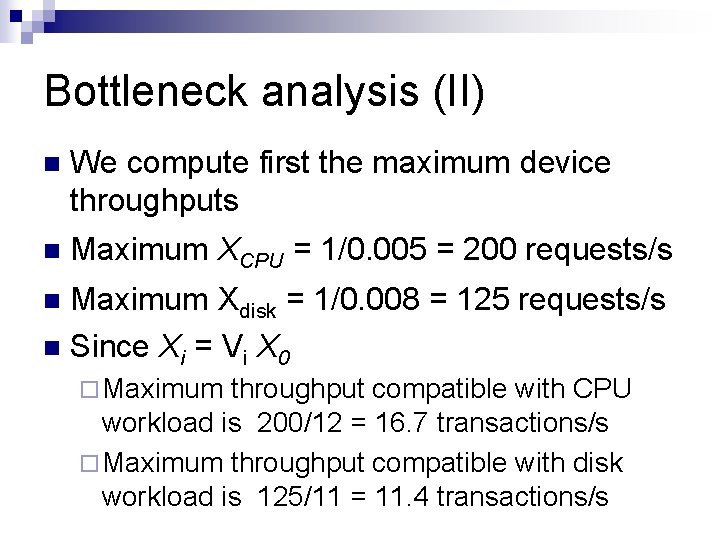
Bottleneck analysis (II) n We compute first the maximum device throughputs n Maximum XCPU = 1/0. 005 = 200 requests/s Maximum Xdisk = 1/0. 008 = 125 requests/s n Since Xi = Vi X 0 n ¨ Maximum throughput compatible with CPU workload is 200/12 = 16. 7 transactions/s ¨ Maximum throughput compatible with disk workload is 125/11 = 11. 4 transactions/s

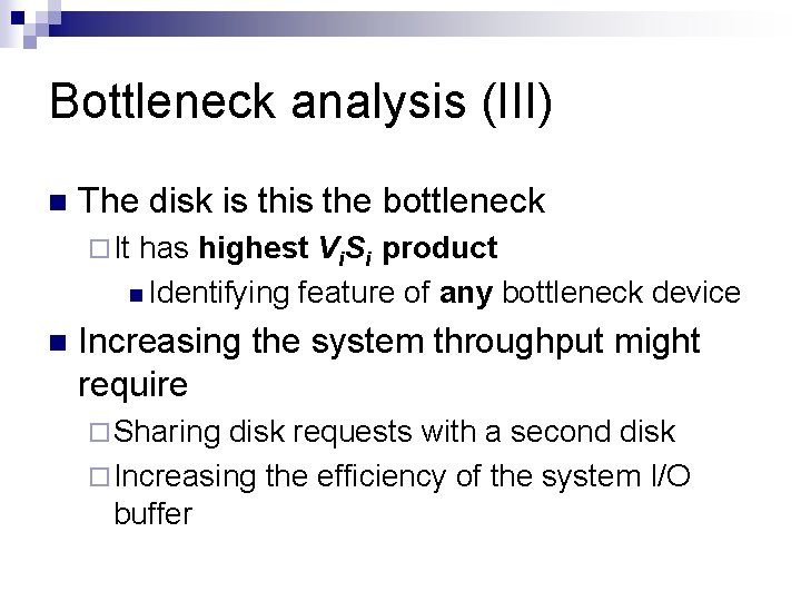
Bottleneck analysis (III) n The disk is the bottleneck ¨ It has highest Vi. Si product n Identifying feature of any bottleneck device n Increasing the system throughput might require ¨ Sharing disk requests with a second disk ¨ Increasing the efficiency of the system I/O buffer

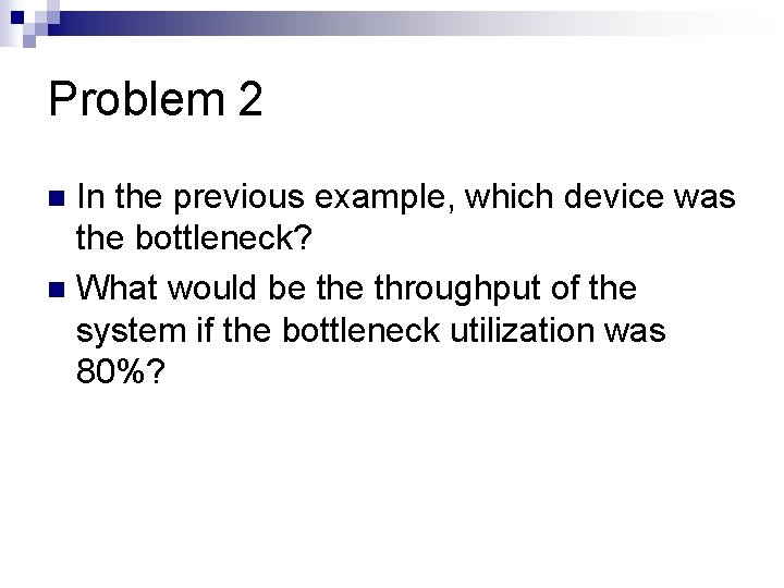
Problem 2 In the previous example, which device was the bottleneck? n What would be throughput of the system if the bottleneck utilization was 80%? n

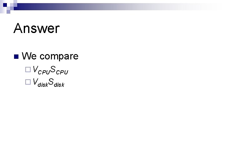
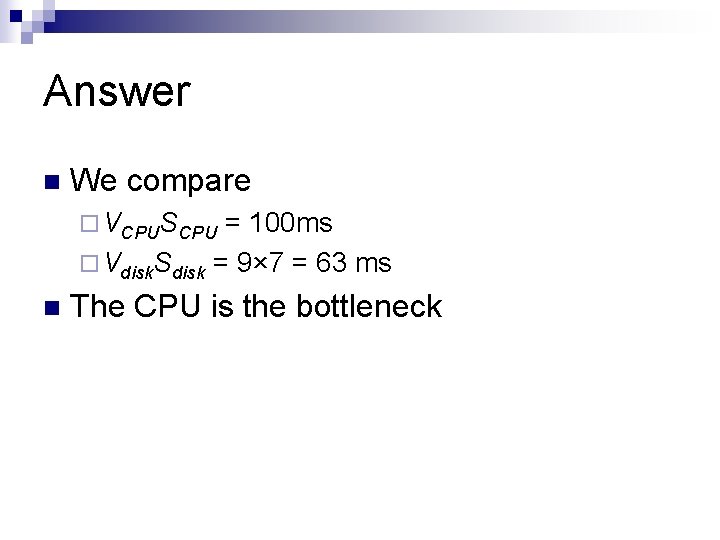
Answer n We compare ¨ VCPUSCPU ¨ Vdisk. Sdisk

Answer n We compare ¨ VCPUSCPU = 100 ms ¨ Vdisk. Sdisk = 9× 7 = 63 ms n The CPU is the bottleneck

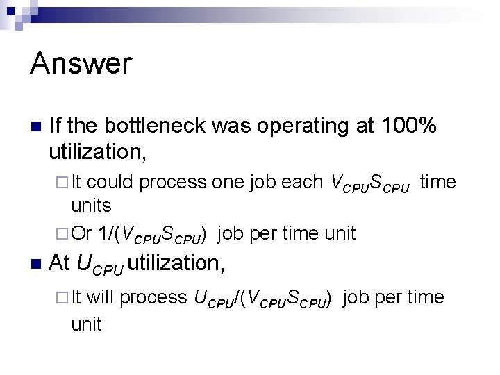
Answer n If the bottleneck was operating at 100% utilization, ¨ It could process one job each VCPUSCPU time units ¨ Or 1/(VCPUSCPU) job per time unit n At UCPU utilization, ¨ It will process UCPU/(VCPUSCPU) job per time unit

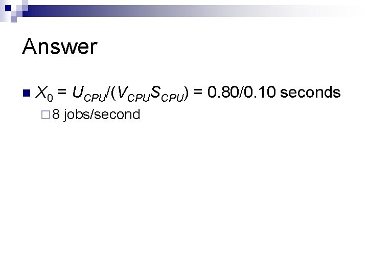
Answer n X 0 = UCPU/(VCPUSCPU) = 0. 80/0. 10 seconds ¨ 8 jobs/second

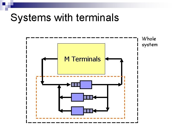
Systems with terminals Whole system M Terminals

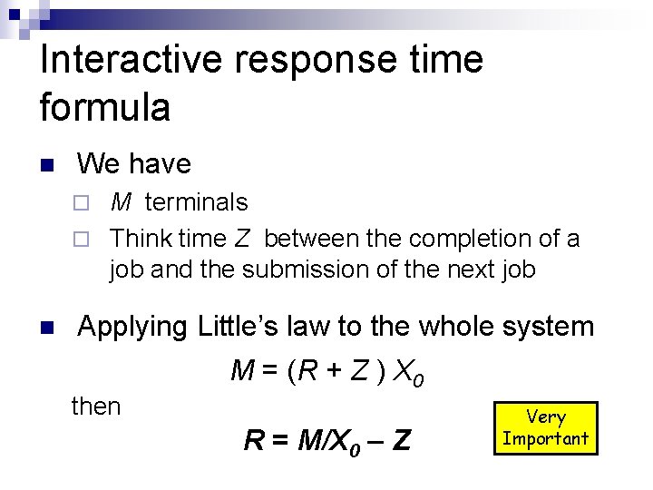
Interactive response time formula n We have M terminals ¨ Think time Z between the completion of a job and the submission of the next job ¨ n Applying Little’s law to the whole system M = (R + Z ) X 0 then R = M/X 0 – Z Very Important

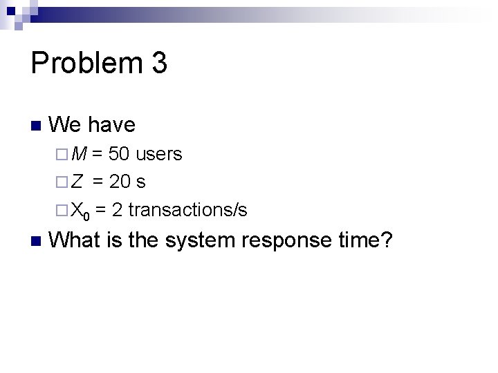
Problem 3 n We have ¨M = 50 users ¨ Z = 20 s ¨ X 0 = 2 transactions/s n What is the system response time?

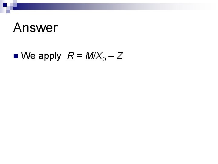
Answer n We apply R = M/X 0 – Z

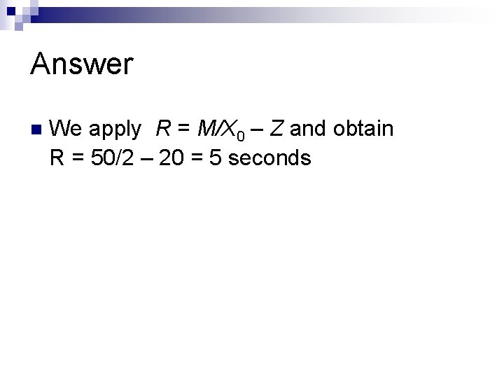
Answer n We apply R = M/X 0 – Z and obtain R = 50/2 – 20 = 5 seconds

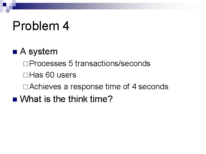
Problem 4 n A system ¨ Processes 5 transactions/seconds ¨ Has 60 users ¨ Achieves a response time of 4 seconds n What is the think time?

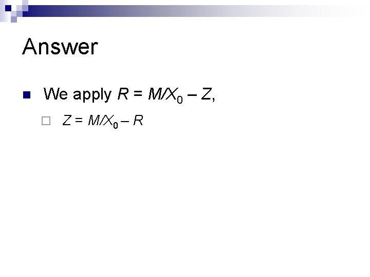
Answer n We apply R = M/X 0 – Z, ¨ Z = M/X 0 – R

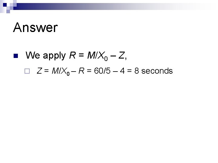
Answer n We apply R = M/X 0 – Z, ¨ Z = M/X 0 – R = 60/5 – 4 = 8 seconds

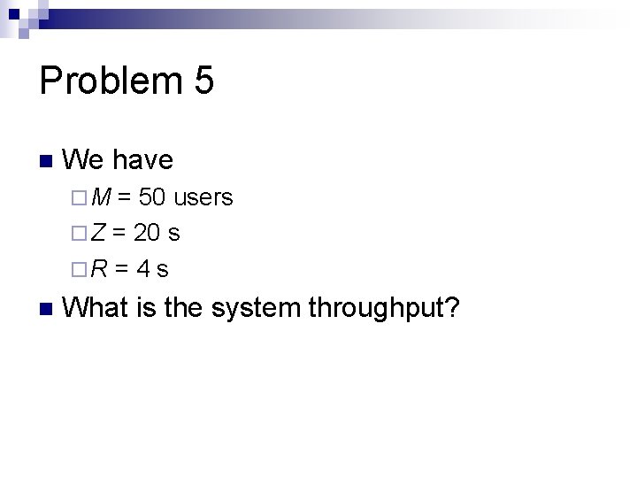
Problem 5 n We have ¨M = 50 users ¨ Z = 20 s ¨R = 4 s n What is the system throughput?

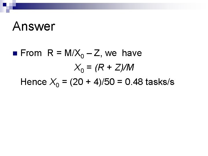
Answer n From R = M/X 0 – Z, we have X 0 = (R + Z)/M Hence X 0 = (20 + 4)/50 = 0. 48 tasks/s

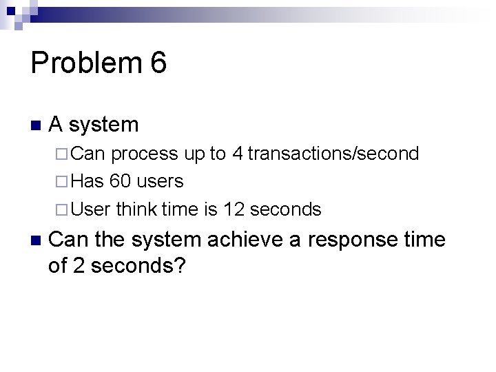
Problem 6 n A system ¨ Can process up to 4 transactions/second ¨ Has 60 users ¨ User think time is 12 seconds n Can the system achieve a response time of 2 seconds?

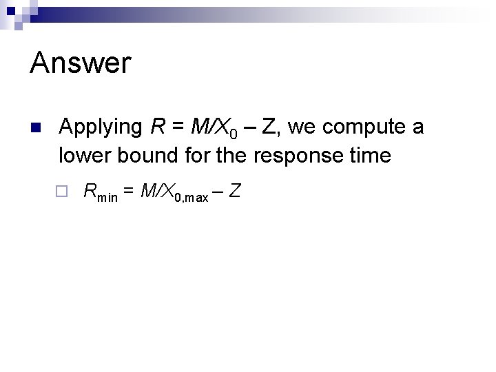
Answer n Applying R = M/X 0 – Z, we compute a lower bound for the response time ¨ Rmin = M/X 0, max – Z

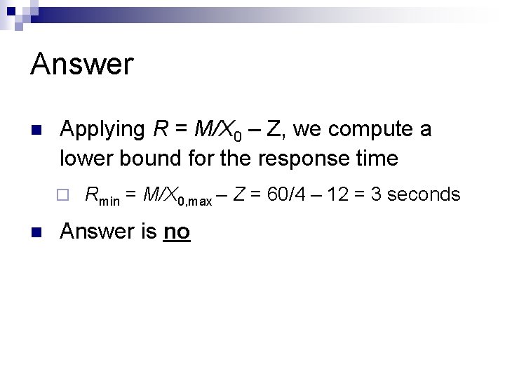
Answer n Applying R = M/X 0 – Z, we compute a lower bound for the response time ¨ n Rmin = M/X 0, max – Z = 60/4 – 12 = 3 seconds Answer is no

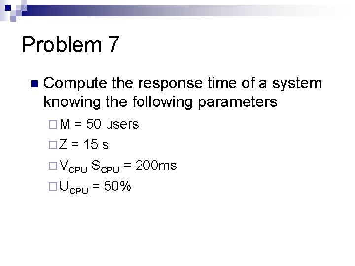
Problem 7 n Compute the response time of a system knowing the following parameters ¨M = 50 users ¨ Z = 15 s ¨ VCPU SCPU = 200 ms ¨ UCPU = 50%

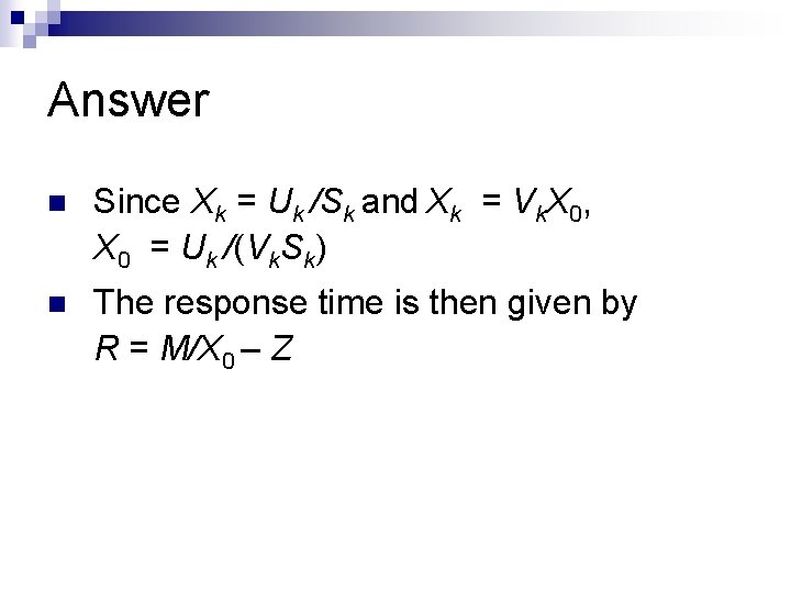
Answer n Since Xk = Uk /Sk and Xk = Vk. X 0, X 0 = Uk /(Vk. Sk) n The response time is then given by R = M/X 0 – Z

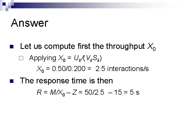
Answer n Let us compute first the throughput X 0 ¨ Applying X 0 = Uk/(Vk. Sk) X 0 = 0. 50/0. 200 = 2. 5 interactions/s n The response time is then R = M/X 0 – Z = 50/2. 5 – 15 = 5 s

Simulation Case Studies

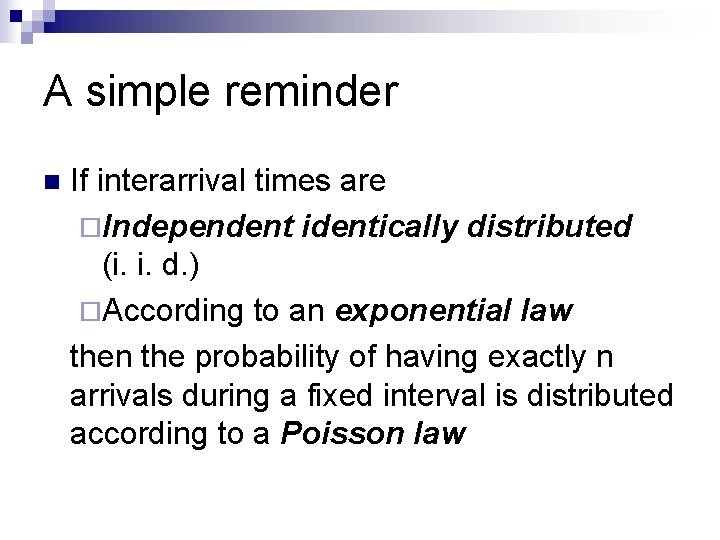
A simple reminder n If interarrival times are ¨Independent identically distributed (i. i. d. ) ¨According to an exponential law then the probability of having exactly n arrivals during a fixed interval is distributed according to a Poisson law

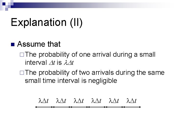
Explanation (II) n Assume that ¨ The probability of one arrival during a small interval Dt is l. Dt ¨ The probability of two arrivals during the same small time interval is negligible l. Dt

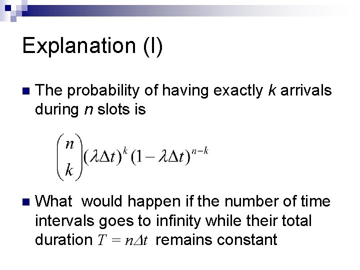
Explanation (I) n The probability of having exactly k arrivals during n slots is n What would happen if the number of time intervals goes to infinity while their total duration T = n. Dt remains constant

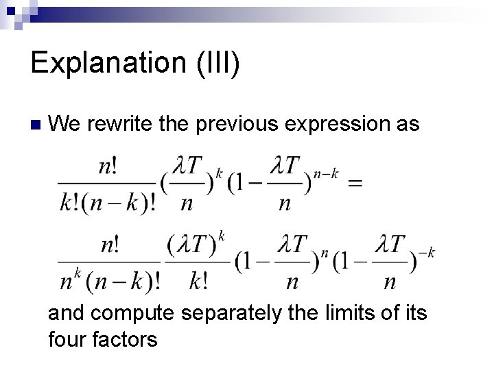
Explanation (III) n We rewrite the previous expression as and compute separately the limits of its four factors

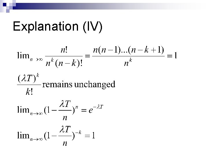
Explanation (IV)

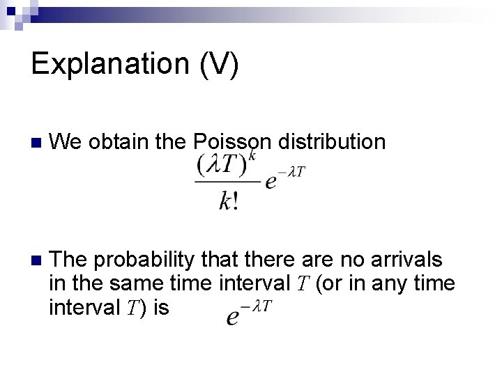
Explanation (V) n We obtain the Poisson distribution n The probability that there are no arrivals in the same time interval T (or in any time interval T) is

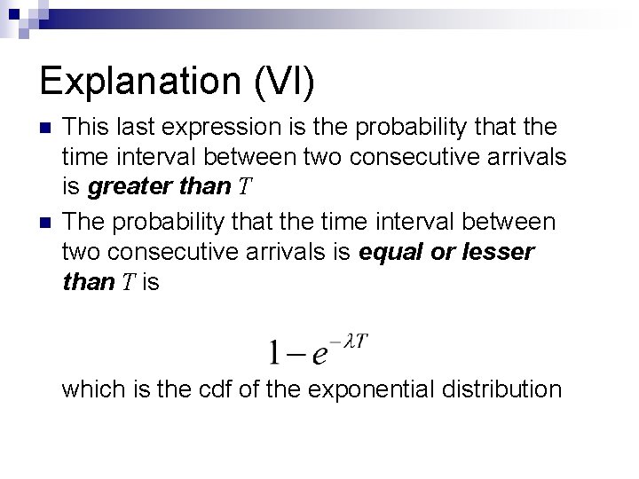
Explanation (VI) n n This last expression is the probability that the time interval between two consecutive arrivals is greater than T The probability that the time interval between two consecutive arrivals is equal or lesser than T is which is the cdf of the exponential distribution

A final observation n Use the Poisson distribution to generate number of arrivals during a time interval n Use the exponential distribution to generate interarrival times

Linear Regression

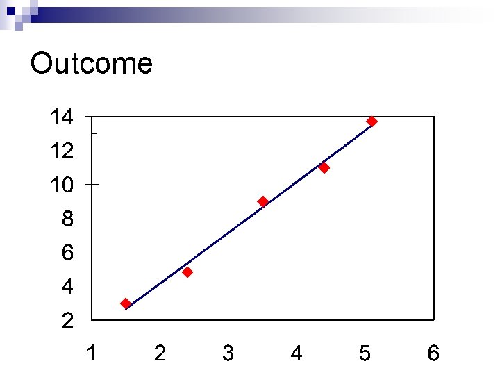
Most important point n Compute a regression line n Compute regression coefficient

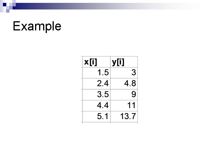
Example

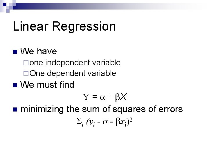
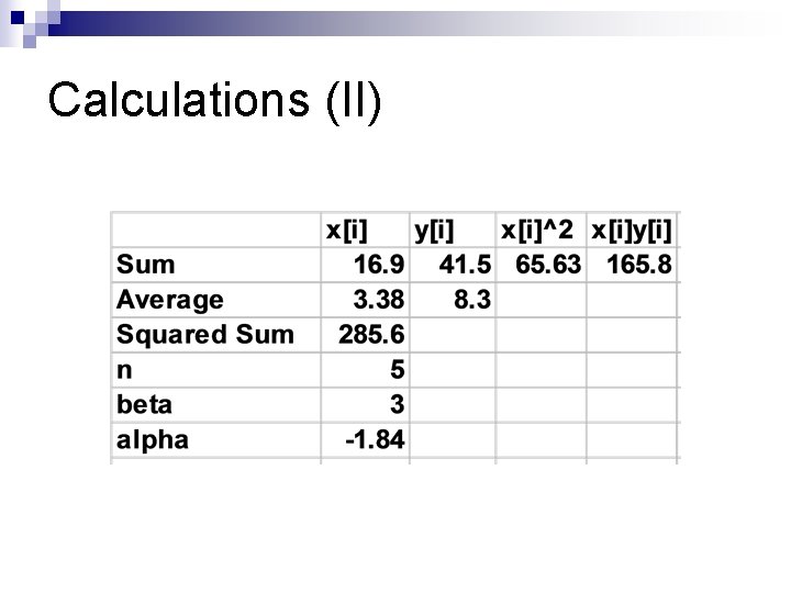
Linear Regression n We have ¨ one independent variable ¨ One dependent variable n We must find Y = + b. X n minimizing the sum of squares of errors Si (yi - - bxi)2

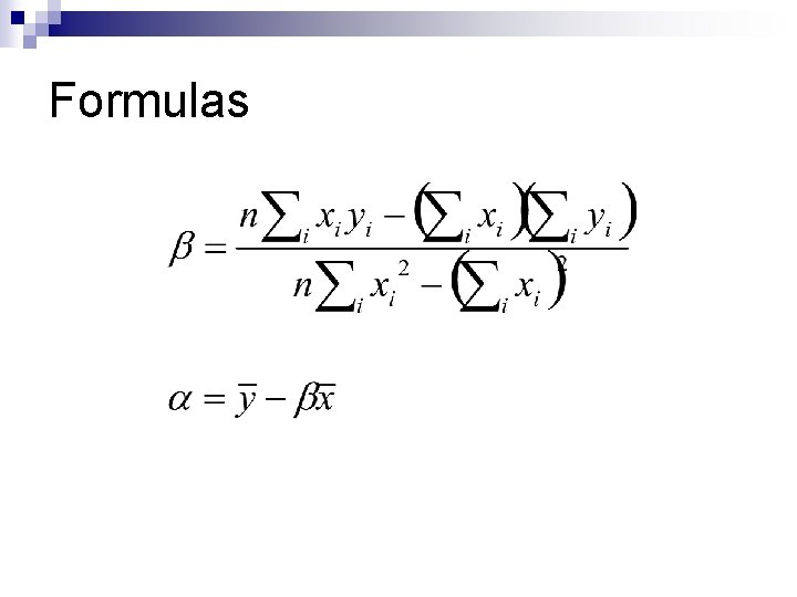
Formulas

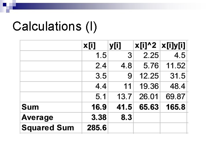
Calculations (I)

Calculations (II)

Outcome

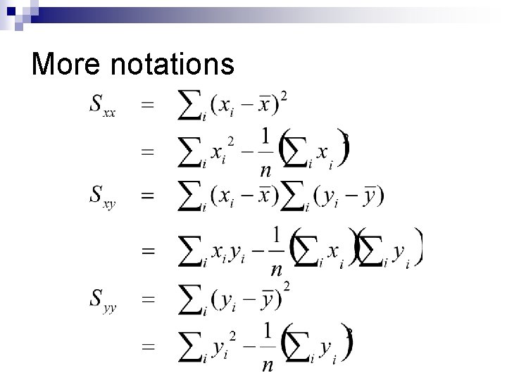
More notations

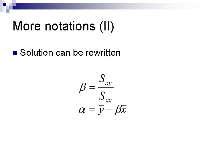
More notations (II) n Solution can be rewritten

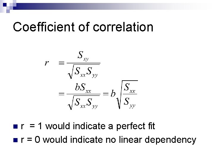
Coefficient of correlation r = 1 would indicate a perfect fit n r = 0 would indicate no linear dependency n

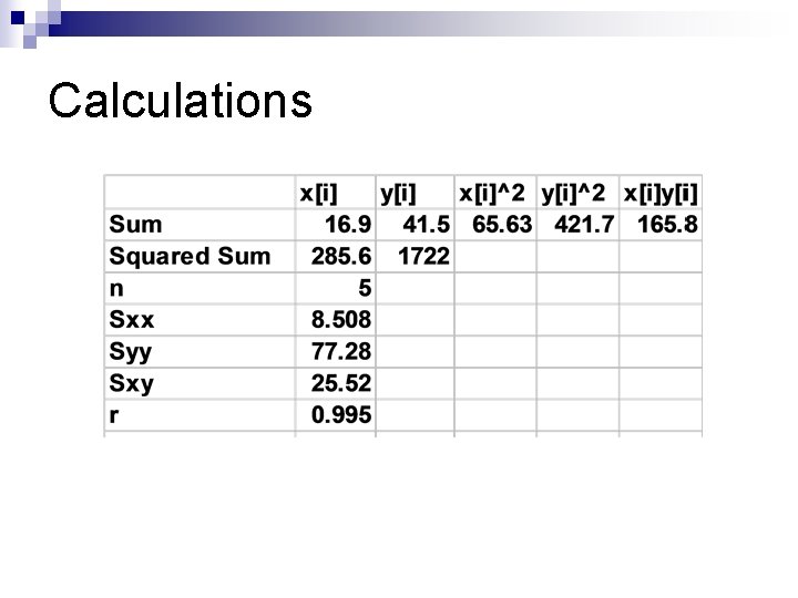
Calculations