Review Session 1 Events during Precipitation Infiltration Not

Review Session 1

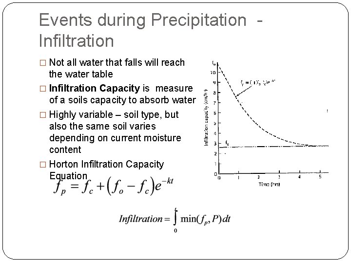
Events during Precipitation Infiltration � Not all water that falls will reach the water table � Infiltration Capacity is measure of a soils capacity to absorb water � Highly variable – soil type, but also the same soil varies depending on current moisture content � Horton Infiltration Capacity Equation

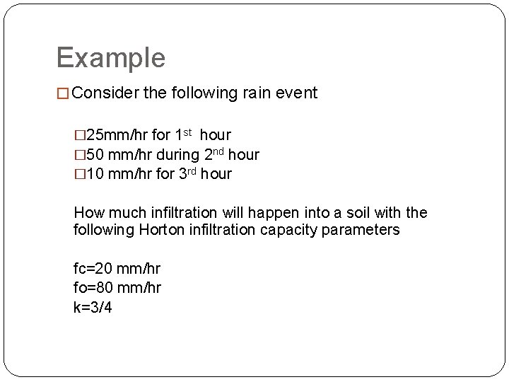
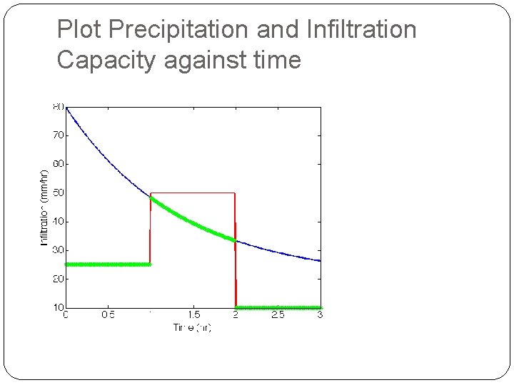
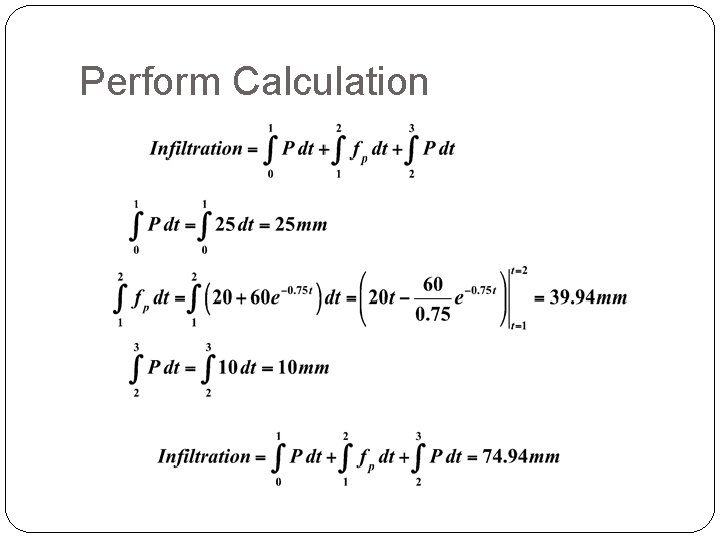
Example � Consider the following rain event � 25 mm/hr for 1 st hour � 50 mm/hr during 2 nd hour � 10 mm/hr for 3 rd hour How much infiltration will happen into a soil with the following Horton infiltration capacity parameters fc=20 mm/hr fo=80 mm/hr k=3/4

Plot Precipitation and Infiltration Capacity against time

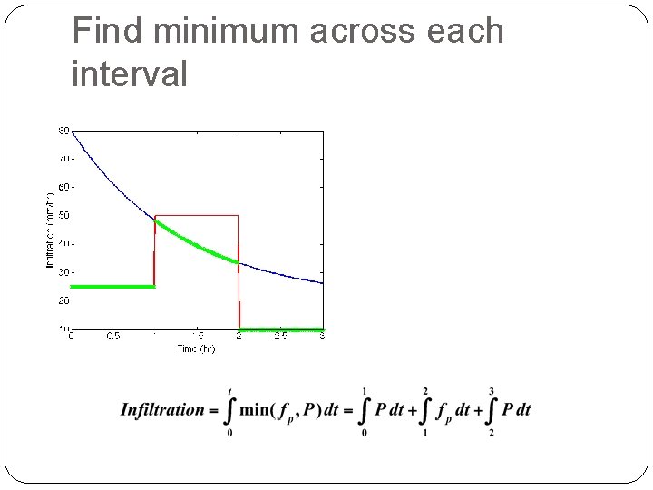
Find minimum across each interval

Perform Calculation

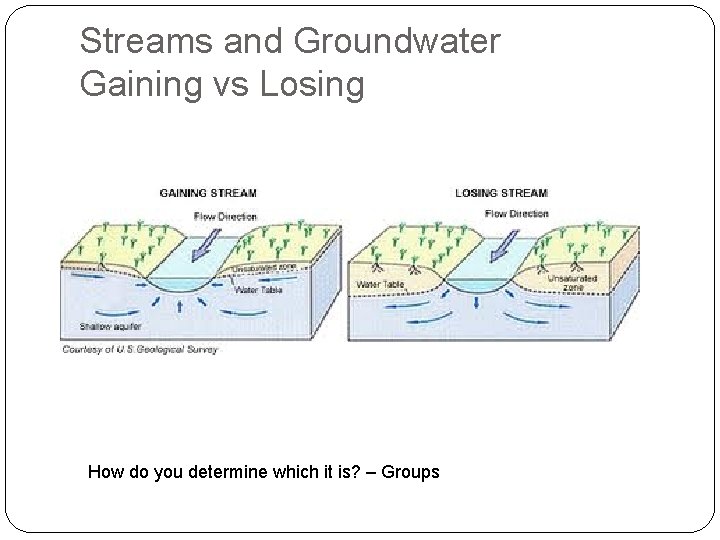
Streams and Groundwater Gaining vs Losing How do you determine which it is? – Groups

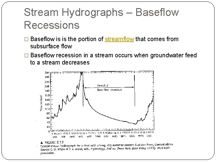
Stream Hydrographs – Baseflow Recessions � Baseflow is is the portion of streamflow that comes from subsurface flow � Baseflow recession in a stream occurs when groundwater feed to a stream decreases

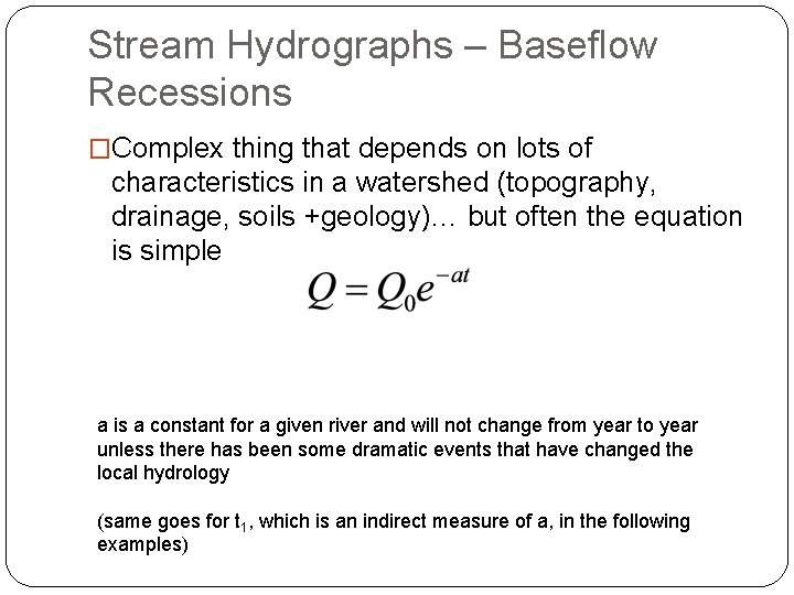
Stream Hydrographs – Baseflow Recessions �Complex thing that depends on lots of characteristics in a watershed (topography, drainage, soils +geology)… but often the equation is simple a is a constant for a given river and will not change from year to year unless there has been some dramatic events that have changed the local hydrology (same goes for t 1, which is an indirect measure of a, in the following examples)

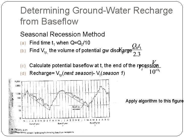
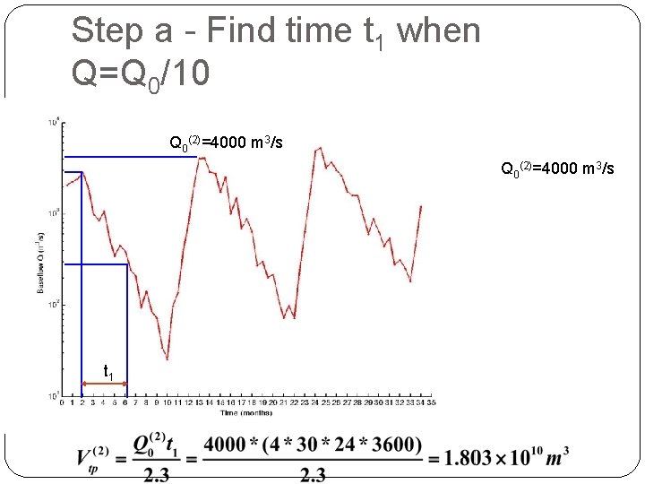
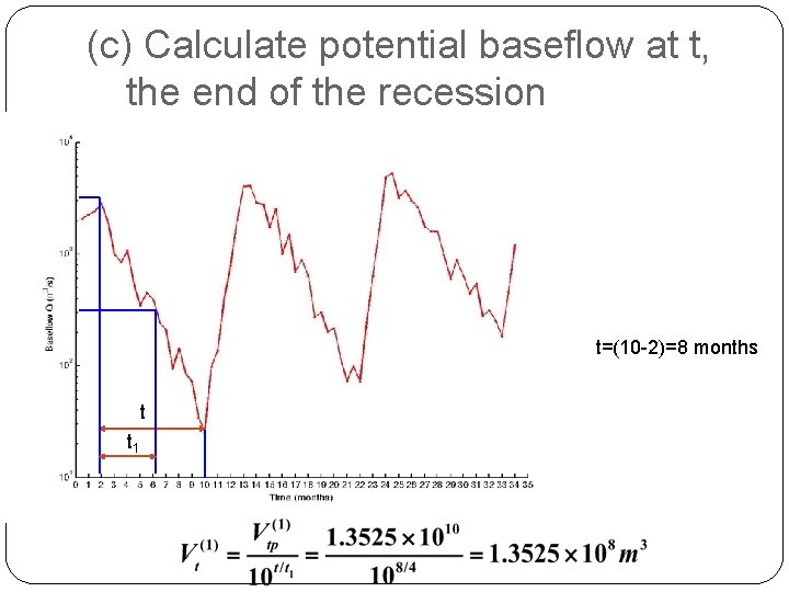
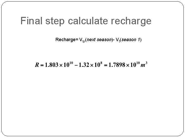
Determining Ground-Water Recharge from Baseflow Seasonal Recession Method (a) Find time t 1 when Q=Q 0/10 (b) Find Vtp, the volume of potential gw discharge (c) Calculate potential baseflow at t, the end of the recession (d) Recharge= Vtp(next season)- Vt(season 1) Apply algorithm to this figure

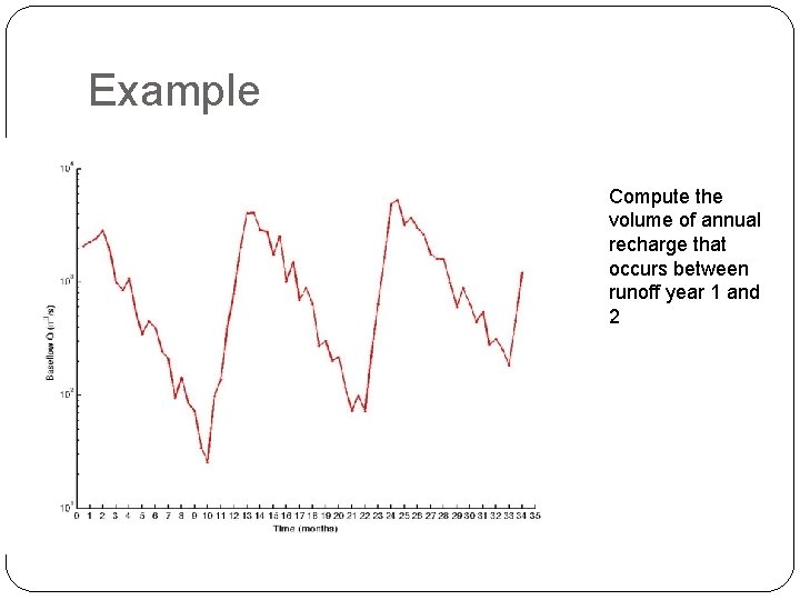
Example Compute the volume of annual recharge that occurs between runoff year 1 and 2

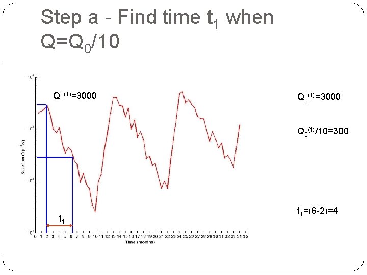
Step a - Find time t 1 when Q=Q 0/10 Q 0(1)=3000 Q 0(1)/10=300 t 1=(6 -2)=4

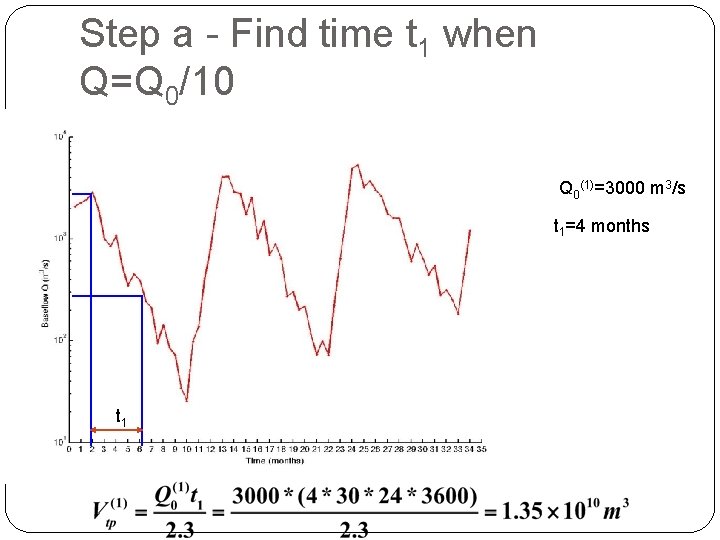
Step a - Find time t 1 when Q=Q 0/10 Q 0(1)=3000 m 3/s t 1=4 months t 1

Step a - Find time t 1 when Q=Q 0/10 Q 0(2)=4000 m 3/s t 1

(c) Calculate potential baseflow at t, the end of the recession t=(10 -2)=8 months t t 1

Final step calculate recharge Recharge= Vtp(next season)- Vt(season 1)

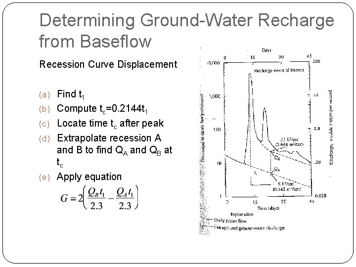
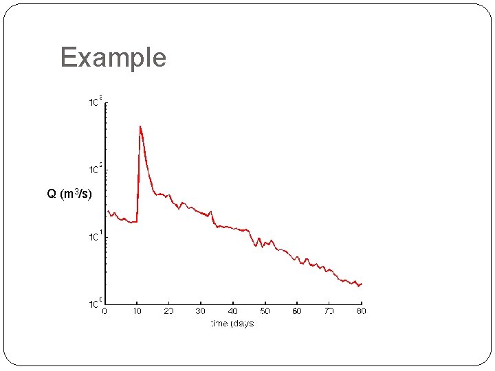
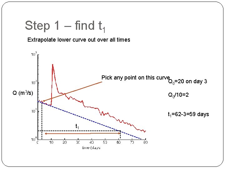
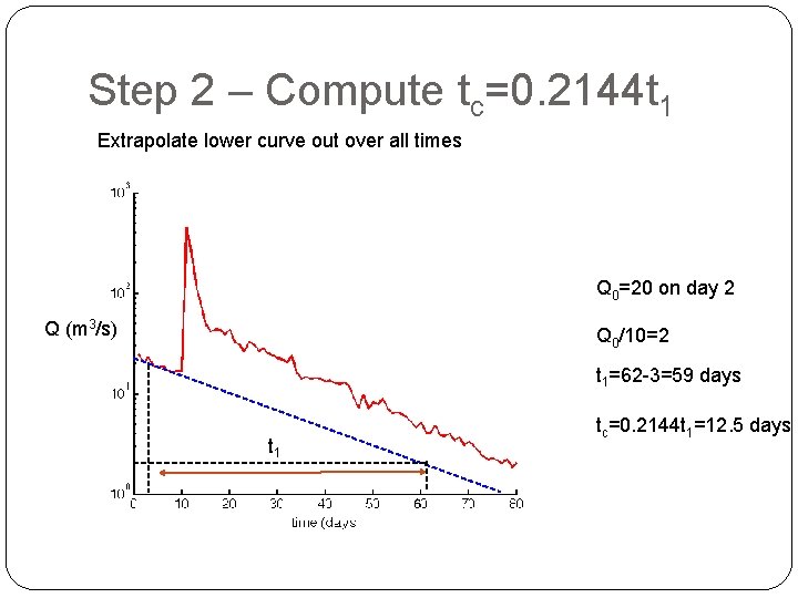
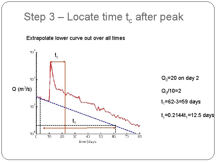
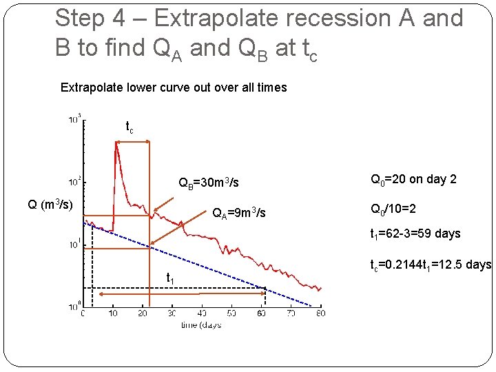
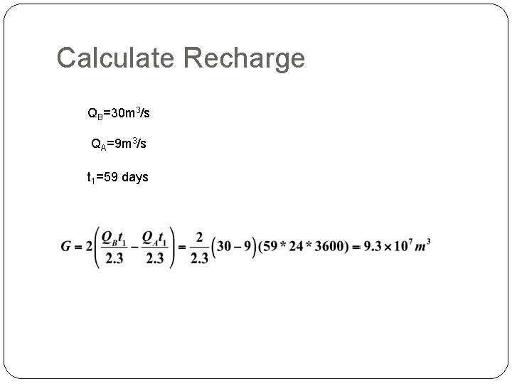
Determining Ground-Water Recharge from Baseflow Recession Curve Displacement (a) Find t 1 (b) Compute tc=0. 2144 t 1 (c) Locate time tc after peak (d) Extrapolate recession A and B to find QA and QB at tc (e) Apply equation

Example Q (m 3/s)

Step 1 – find t 1 Extrapolate lower curve out over all times Pick any point on this curve Q 0=20 on day 3 Q (m 3/s) Q 0/10=2 t 1=62 -3=59 days t 1

Step 2 – Compute tc=0. 2144 t 1 Extrapolate lower curve out over all times Q 0=20 on day 2 Q (m 3/s) Q 0/10=2 t 1=62 -3=59 days t 1 tc=0. 2144 t 1=12. 5 days

Step 3 – Locate time tc after peak Extrapolate lower curve out over all times tc Q 0=20 on day 2 Q (m 3/s) Q 0/10=2 t 1=62 -3=59 days t 1 tc=0. 2144 t 1=12. 5 days

Step 4 – Extrapolate recession A and B to find QA and QB at tc Extrapolate lower curve out over all times tc QB=30 m 3/s Q (m 3/s) QA=9 m 3/s Q 0=20 on day 2 Q 0/10=2 t 1=62 -3=59 days t 1 tc=0. 2144 t 1=12. 5 days

Calculate Recharge QB=30 m 3/s QA=9 m 3/s t 1=59 days

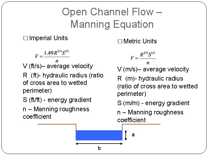
Open Channel Flow – Manning Equation � Imperial Units � Metric Units V (ft/s)– average velocity R (ft)- hydraulic radius (ratio of cross area to wetted perimeter) S (ft/ft) - energy gradient n – Manning roughness coefficient V (m/s)– average velocity R (m)- hydraulic radius (ratio of cross area to wetted perimeter) S (m/m) - energy gradient n – Manning roughness coefficient a b

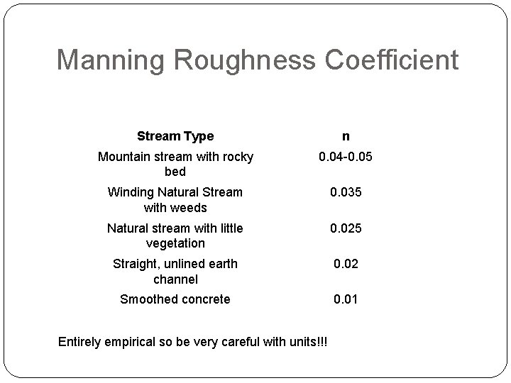
Manning Roughness Coefficient Stream Type n Mountain stream with rocky bed 0. 04 -0. 05 Winding Natural Stream with weeds 0. 035 Natural stream with little vegetation 0. 025 Straight, unlined earth channel 0. 02 Smoothed concrete 0. 01 Entirely empirical so be very careful with units!!!

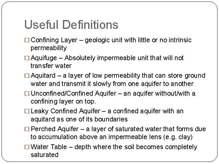
Useful Definitions � Confining Layer – geologic unit with little or no intrinsic permeability � Aquifuge – Absolutely impermeable unit that will not transfer water � Aquitard – a layer of low permeability that can store ground water and transmit it slowly from one aquifer to another � Unconfined/Confined Aquifer – an aquifer without/with a confining layer on top. � Leaky Confined Aquifer – a confined aquifer with an aquitard as one of its boundaries � Perched Aquifer – a layer of saturated water that forms due to accumulation above an impermeable lens (e. g. clay) � Water Table – depth where the soil becomes completely saturated

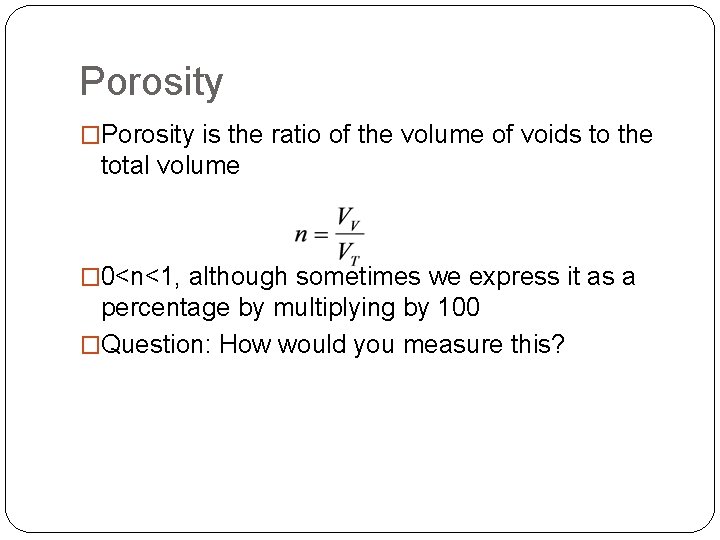
Porosity �Porosity is the ratio of the volume of voids to the total volume � 0<n<1, although sometimes we express it as a percentage by multiplying by 100 �Question: How would you measure this?

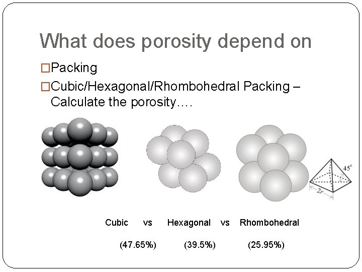
What does porosity depend on �Packing �Cubic/Hexagonal/Rhombohedral Packing – Calculate the porosity…. Cubic vs (47. 65%) Hexagonal (39. 5%) vs Rhombohedral (25. 95%)

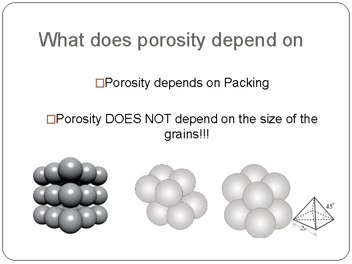
What does porosity depend on �Porosity depends on Packing �Porosity DOES NOT depend on the size of the grains!!!

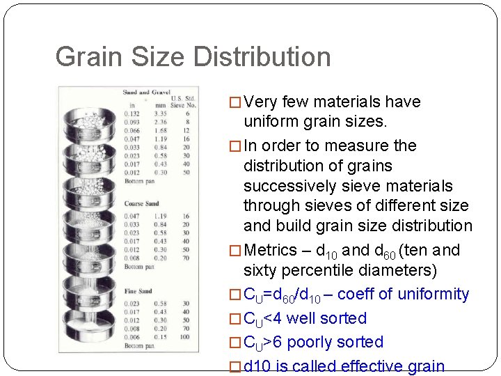
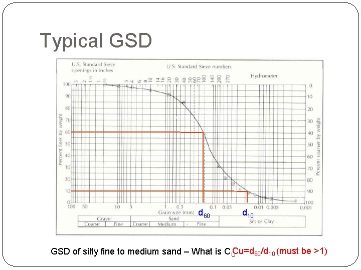
Grain Size Distribution � Very few materials have uniform grain sizes. � In order to measure the distribution of grains successively sieve materials through sieves of different size and build grain size distribution � Metrics – d 10 and d 60 (ten and sixty percentile diameters) � CU=d 60/d 10 – coeff of uniformity � CU<4 well sorted � CU>6 poorly sorted � d 10 is called effective grain

Typical GSD d 60 d 10 GSD of silty fine to medium sand – What is CUCu=d 60/d 10 (must be >1)

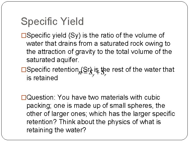
Specific Yield �Specific yield (Sy) is the ratio of the volume of water that drains from a saturated rock owing to the attraction of gravity to the total volume of the saturated aquifer. �Specific retention (Sr) is the rest of the water that is retained �Question: You have two materials with cubic packing; one is made up of small spheres, the other of larger ones; which has the larger specific retention? Think about the physics of what is retaining the water?

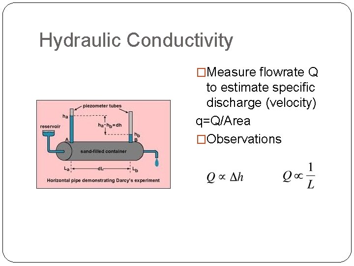
Hydraulic Conductivity �Measure flowrate Q to estimate specific discharge (velocity) q=Q/Area �Observations

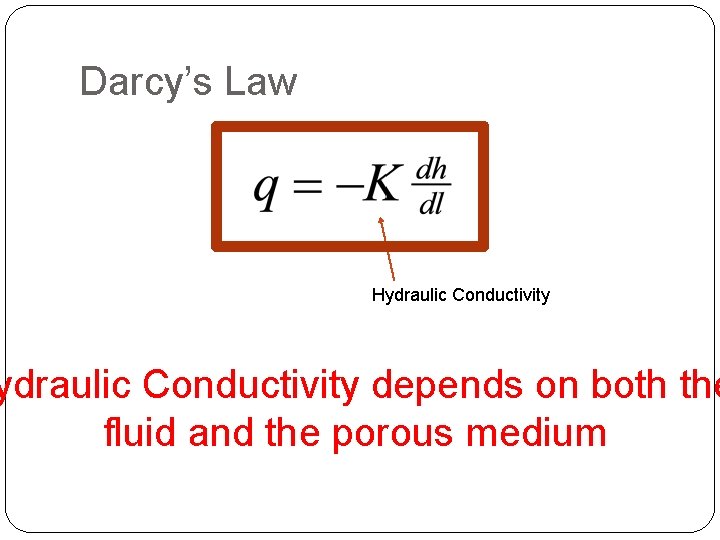
Darcy’s Law Hydraulic Conductivity depends on both the fluid and the porous medium

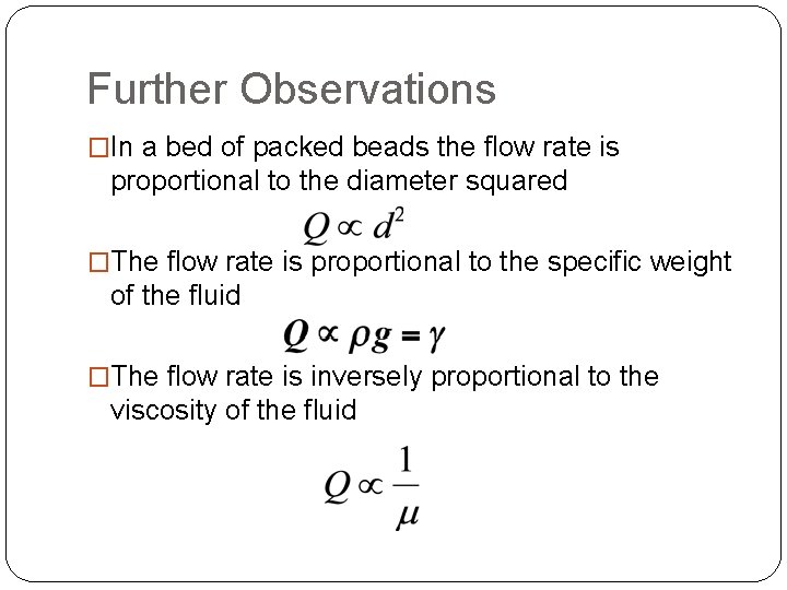
Further Observations �In a bed of packed beads the flow rate is proportional to the diameter squared �The flow rate is proportional to the specific weight of the fluid �The flow rate is inversely proportional to the viscosity of the fluid

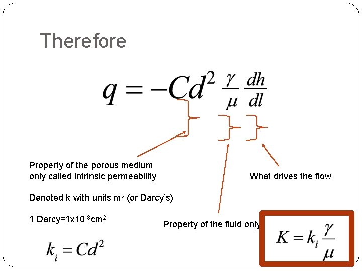
Therefore Property of the porous medium only called intrinsic permeability What drives the flow Denoted ki with units m 2 (or Darcy’s) 1 Darcy=1 x 10 -8 cm 2 Property of the fluid only

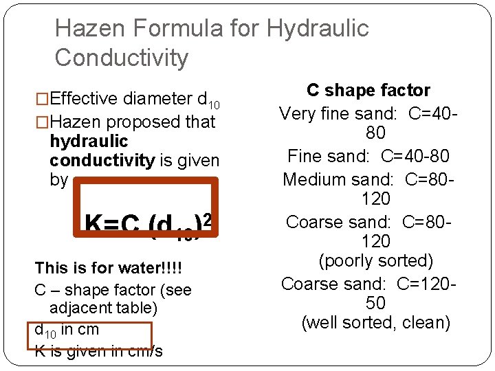
Hazen Formula for Hydraulic Conductivity �Effective diameter d 10 �Hazen proposed that hydraulic conductivity is given by K=C (d 10)2 This is for water!!!! C – shape factor (see adjacent table) d 10 in cm K is given in cm/s C shape factor Very fine sand: C=4080 Fine sand: C=40 -80 Medium sand: C=80120 Coarse sand: C=80120 (poorly sorted) Coarse sand: C=12050 (well sorted, clean)

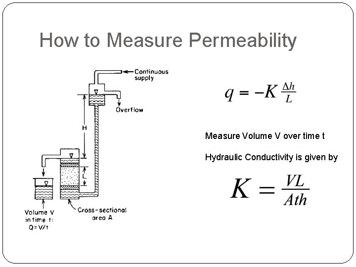
How to Measure Permeability Measure Volume V over time t Hydraulic Conductivity is given by

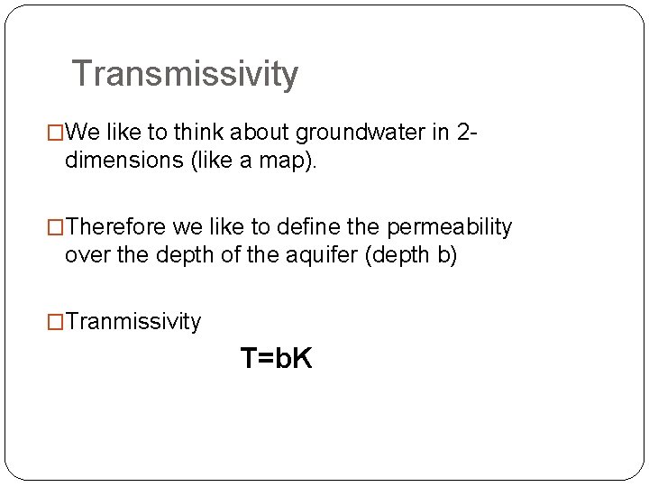
Transmissivity �We like to think about groundwater in 2 - dimensions (like a map). �Therefore we like to define the permeability over the depth of the aquifer (depth b) �Tranmissivity T=b. K

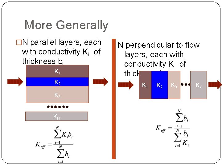
More Generally �N parallel layers, each with conductivity Ki of thickness bi K 1 K 2 K 3 KN N perpendicular to flow layers, each with conductivity Ki of thickness bi K 1 K 2 K 3 K 4

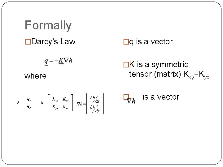
Formally �Darcy’s Law �q is a vector �K is a symmetric where tensor (matrix) Kxy=Kyx � is a vector

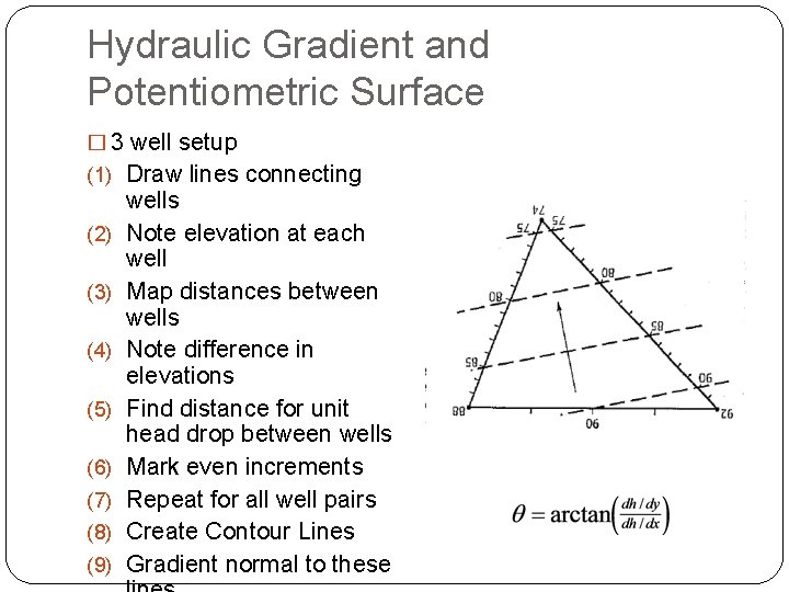
Hydraulic Gradient and Potentiometric Surface � 3 well setup (1) Draw lines connecting (2) (3) (4) (5) (6) (7) (8) (9) wells Note elevation at each well Map distances between wells Note difference in elevations Find distance for unit head drop between wells Mark even increments Repeat for all well pairs Create Contour Lines Gradient normal to these

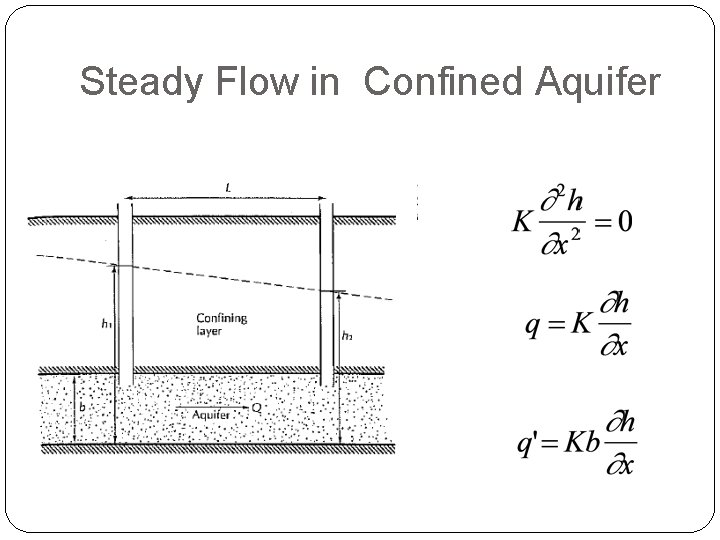
Steady Flow in Confined Aquifer

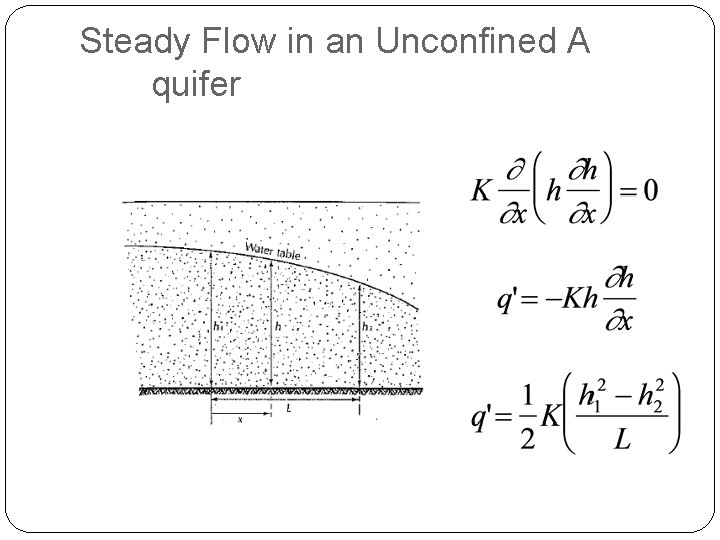
Steady Flow in an Unconfined A quifer

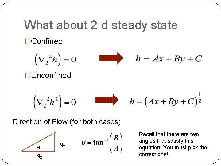
What about 2 -d steady state �Confined �Unconfined Direction of Flow (for both cases) q qx qy Recall that there are two angles that satisfy this equation. You must pick the correct one!

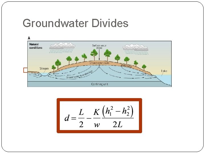
Groundwater Divides �Location of GW Divide is where q’=0

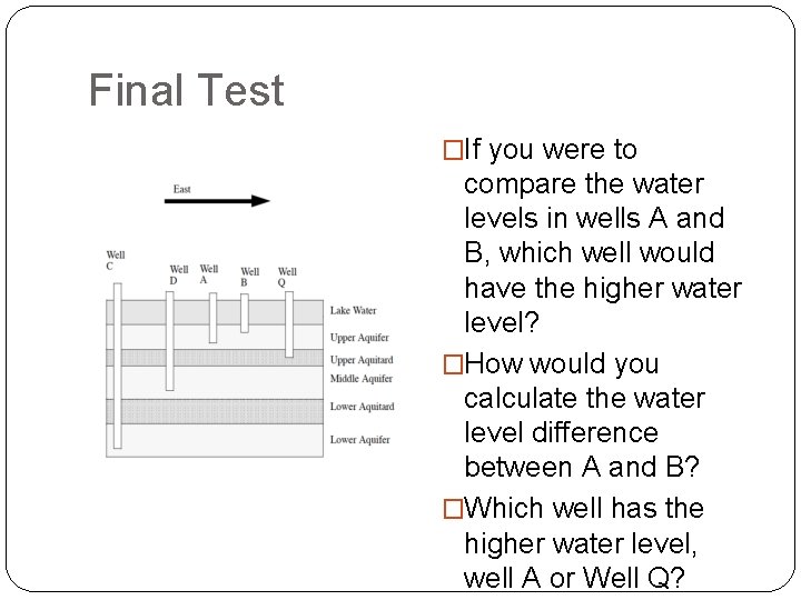
Final Test �If you were to compare the water levels in wells A and B, which well would have the higher water level? �How would you calculate the water level difference between A and B? �Which well has the higher water level, well A or Well Q?