Review Search problem formulation Initial state Actions Transition
Review: Search problem formulation • • • Initial state Actions Transition model Goal state Path cost • What is the optimal solution? • What is the state space?
Review: Tree search • Initialize the fringe using the starting state • While the fringe is not empty – Choose a fringe node to expand according to search strategy – If the node contains the goal state, return solution – Else expand the node and add its children to the fringe
Search strategies • A search strategy is defined by picking the order of node expansion • Strategies are evaluated along the following dimensions: – – Completeness: does it always find a solution if one exists? Optimality: does it always find a least-cost solution? Time complexity: number of nodes generated Space complexity: maximum number of nodes in memory • Time and space complexity are measured in terms of – b: maximum branching factor of the search tree – d: depth of the optimal solution – m: maximum length of any path in the state space (may be infinite)
Uninformed search strategies • Uninformed search strategies use only the information available in the problem definition • • Breadth-first search Uniform-cost search Depth-first search Iterative deepening search
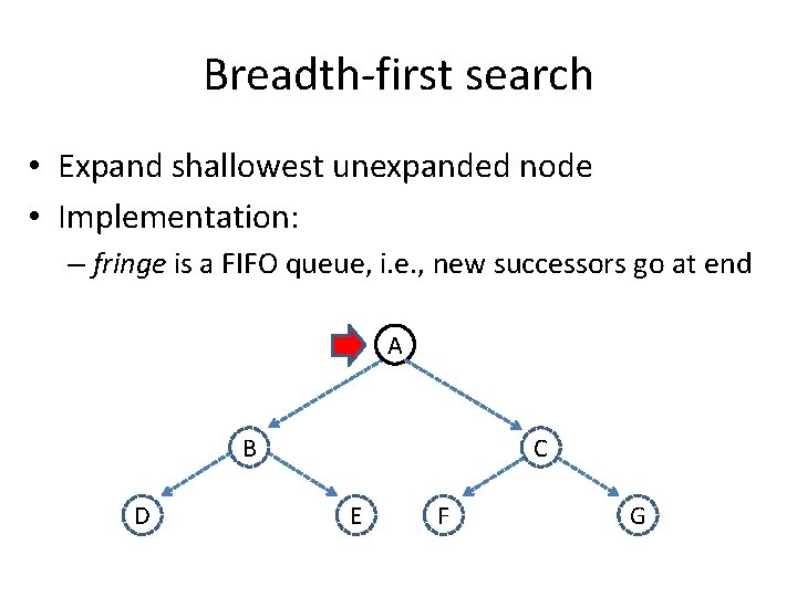
Breadth-first search • Expand shallowest unexpanded node • Implementation: – fringe is a FIFO queue, i. e. , new successors go at end A B D C E F G
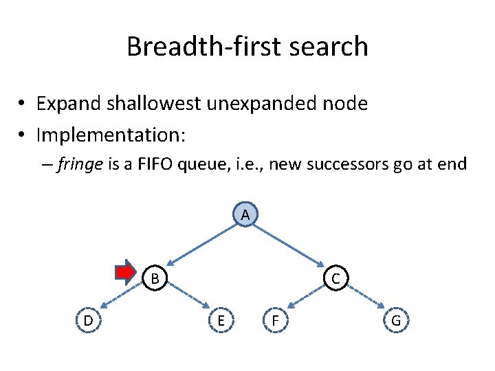
Breadth-first search • Expand shallowest unexpanded node • Implementation: – fringe is a FIFO queue, i. e. , new successors go at end A B D C E F G
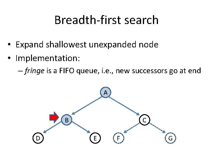
Breadth-first search • Expand shallowest unexpanded node • Implementation: – fringe is a FIFO queue, i. e. , new successors go at end A B D C E F G

Breadth-first search • Expand shallowest unexpanded node • Implementation: – fringe is a FIFO queue, i. e. , new successors go at end A B D C E F G
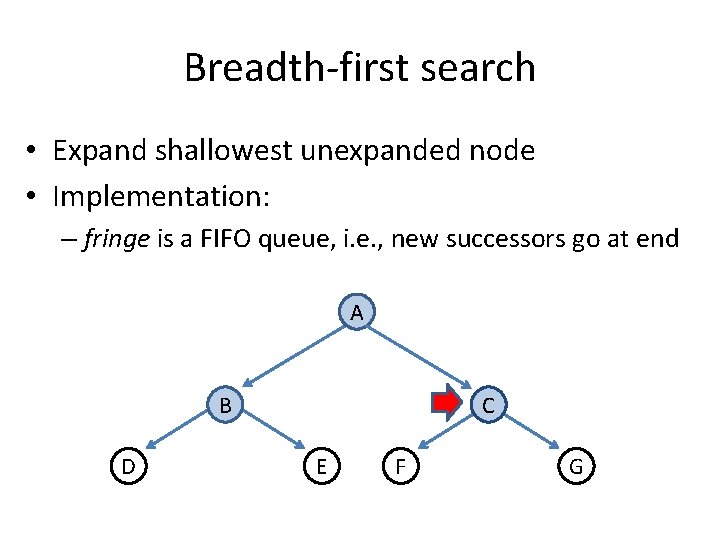
Breadth-first search • Expand shallowest unexpanded node • Implementation: – fringe is a FIFO queue, i. e. , new successors go at end A B D C E F G
Properties of breadth-first search • Complete? Yes (if branching factor b is finite) • Optimal? Yes – if cost = 1 per step • Time? Number of nodes in a b-ary tree of depth d: O(bd) (d is the depth of the optimal solution) • Space? O(bd) • Space is the bigger problem (more than time)
Uniform-cost search • Expand least-cost unexpanded node • Implementation: fringe is a queue ordered by path cost (priority queue) • Equivalent to breadth-first if step costs all equal • Complete? Yes, if step cost is greater than some positive constant ε • Optimal? Yes – nodes expanded in increasing order of path cost • Time? Number of nodes with path cost ≤ cost of optimal solution (C*), O(b. C*/ ε) This can be greater than O(bd): the search can explore long paths consisting of small steps before exploring shorter paths consisting of larger steps • Space? O(b. C*/ ε)
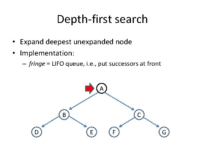
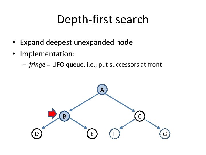
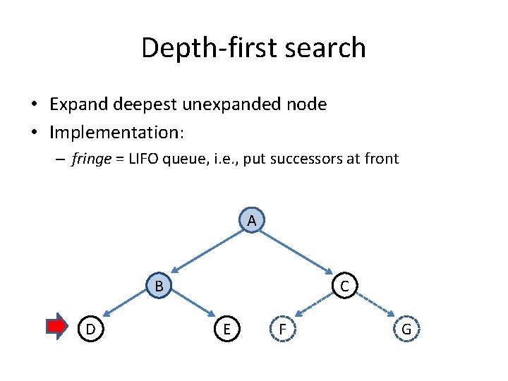
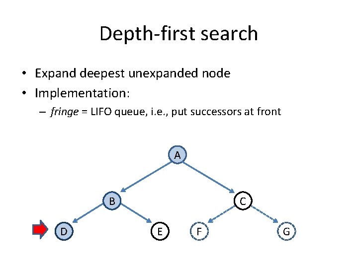
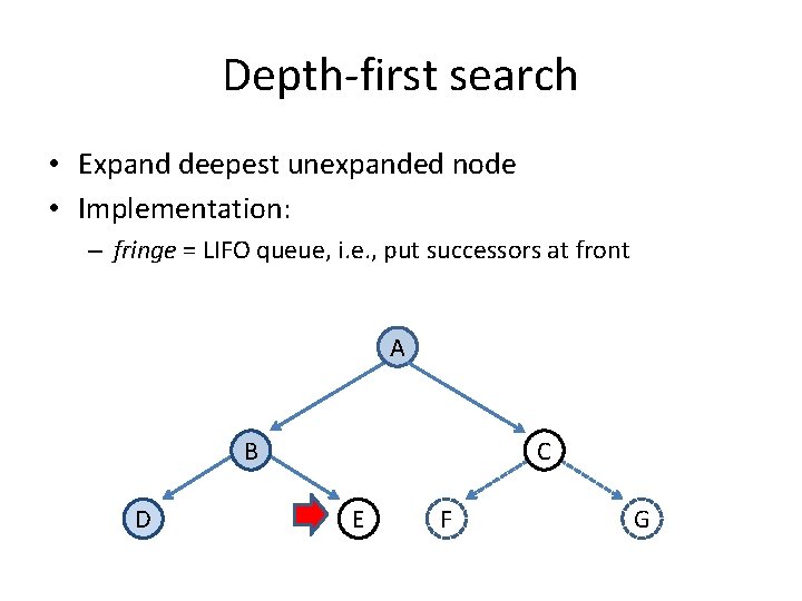
Depth-first search • Expand deepest unexpanded node • Implementation: – fringe = LIFO queue, i. e. , put successors at front A B D C E F G
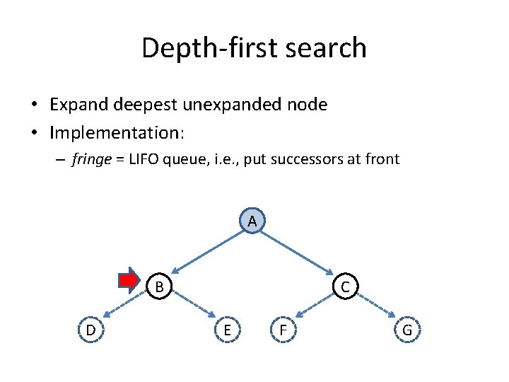
Depth-first search • Expand deepest unexpanded node • Implementation: – fringe = LIFO queue, i. e. , put successors at front A B D C E F G
Depth-first search • Expand deepest unexpanded node • Implementation: – fringe = LIFO queue, i. e. , put successors at front A B D C E F G
Depth-first search • Expand deepest unexpanded node • Implementation: – fringe = LIFO queue, i. e. , put successors at front A B D C E F G
Depth-first search • Expand deepest unexpanded node • Implementation: – fringe = LIFO queue, i. e. , put successors at front A B D C E F G
Depth-first search • Expand deepest unexpanded node • Implementation: – fringe = LIFO queue, i. e. , put successors at front A B D C E F G
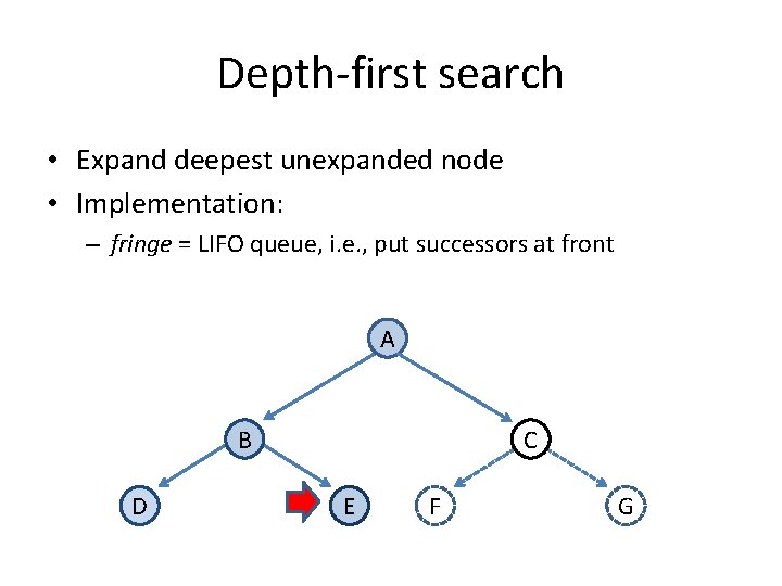
Depth-first search • Expand deepest unexpanded node • Implementation: – fringe = LIFO queue, i. e. , put successors at front A B D C E F G
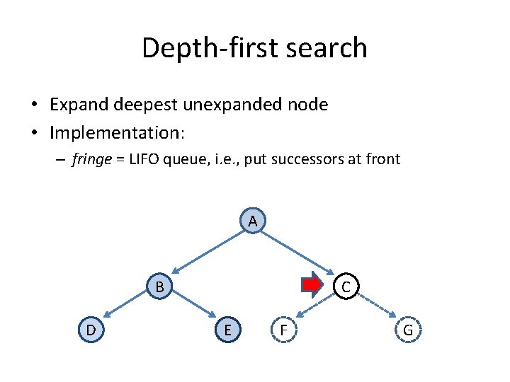
Depth-first search • Expand deepest unexpanded node • Implementation: – fringe = LIFO queue, i. e. , put successors at front A B D C E F G
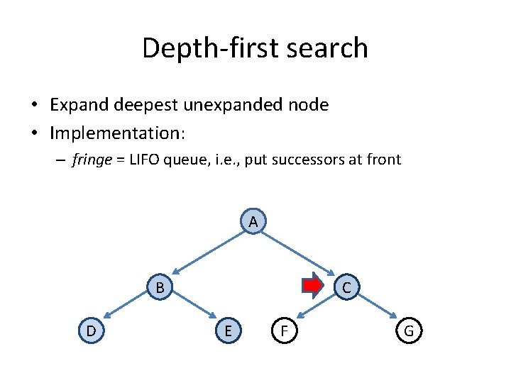
Depth-first search • Expand deepest unexpanded node • Implementation: – fringe = LIFO queue, i. e. , put successors at front A B D C E F G
Properties of depth-first search • Complete? Fails in infinite-depth spaces, spaces with loops Modify to avoid repeated states along path complete in finite spaces • Optimal? No – returns the first solution it finds • Time? Could be the time to reach a solution at maximum depth m: O(bm) Terrible if m is much larger than d But if there are lots of solutions, may be much faster than BFS • Space? O(bm), i. e. , linear space!
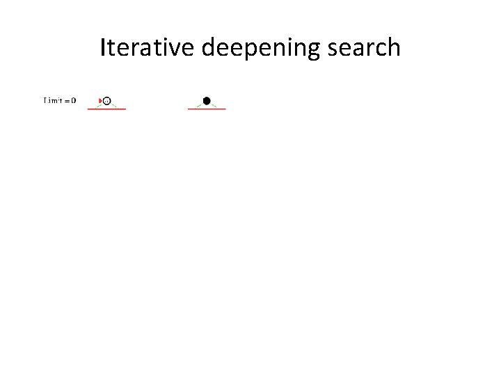
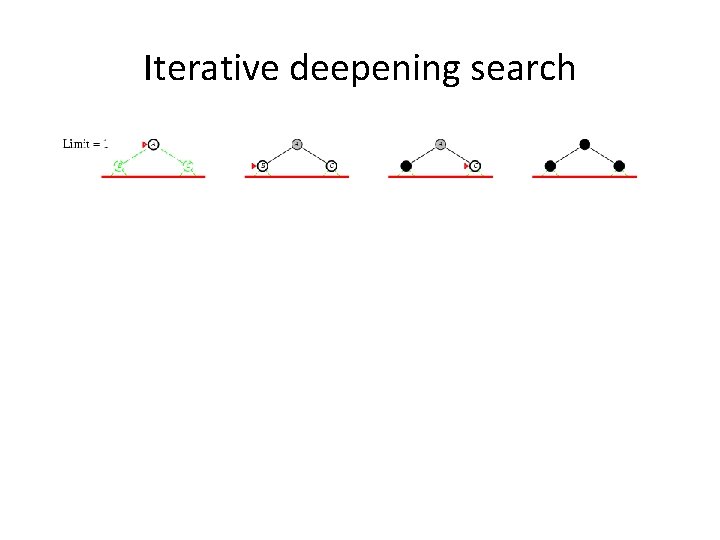
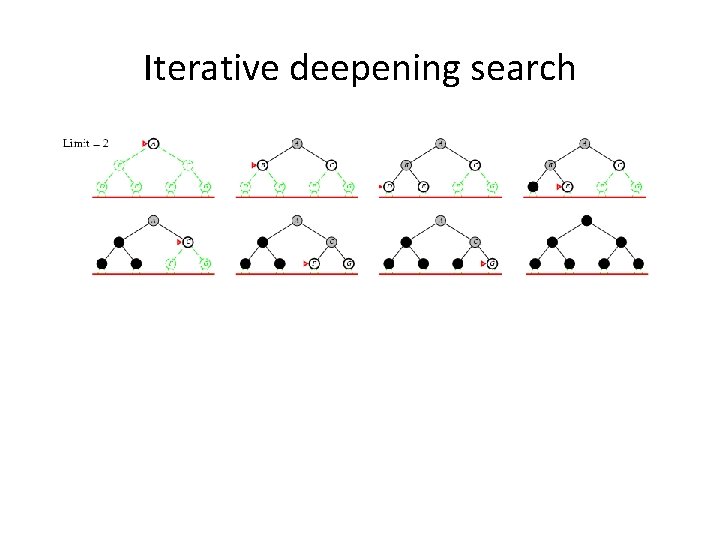
Iterative deepening search • Use DFS as a subroutine 1. Check the root 2. Do a DFS searching for a path of length 1 3. If there is no path of length 1, do a DFS searching for a path of length 2 4. If there is no path of length 2, do a DFS searching for a path of length 3…
Iterative deepening search
Iterative deepening search
Iterative deepening search
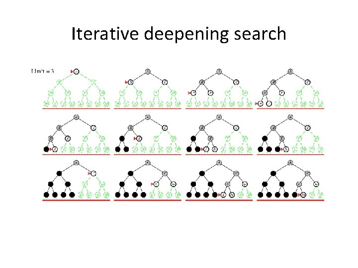
Iterative deepening search
Properties of iterative deepening search • Complete? Yes • Optimal? Yes, if step cost = 1 • Time? (d+1)b 0 + d b 1 + (d-1)b 2 + … + bd = O(bd) • Space? O(bd)
Informed search • Idea: give the algorithm “hints” about the desirability of different states – Use an evaluation function to rank nodes and select the most promising one for expansion • Greedy best-first search • A* search
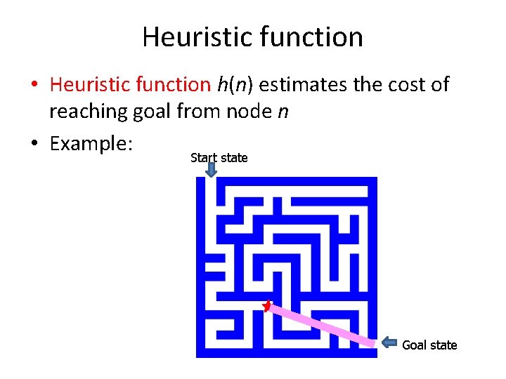
Heuristic function • Heuristic function h(n) estimates the cost of reaching goal from node n • Example: Start state Goal state
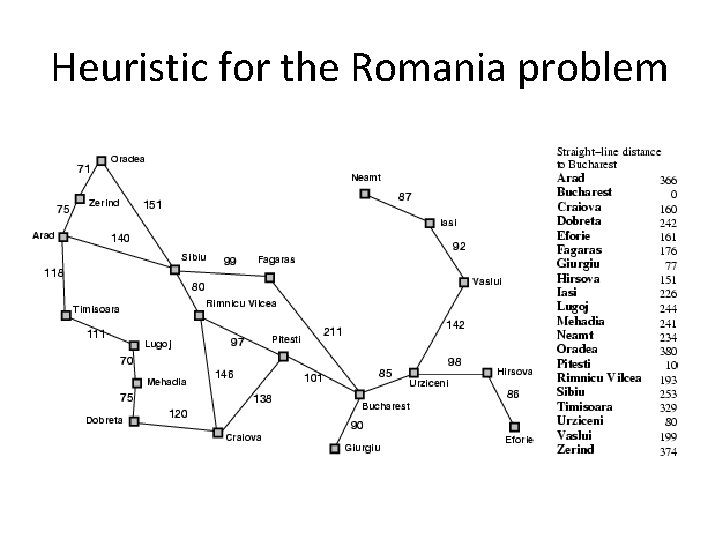
Heuristic for the Romania problem
Greedy best-first search • Expand the node that has the lowest value of the heuristic function h(n)
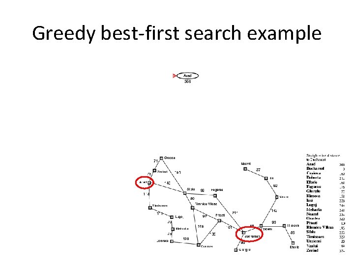
Greedy best-first search example
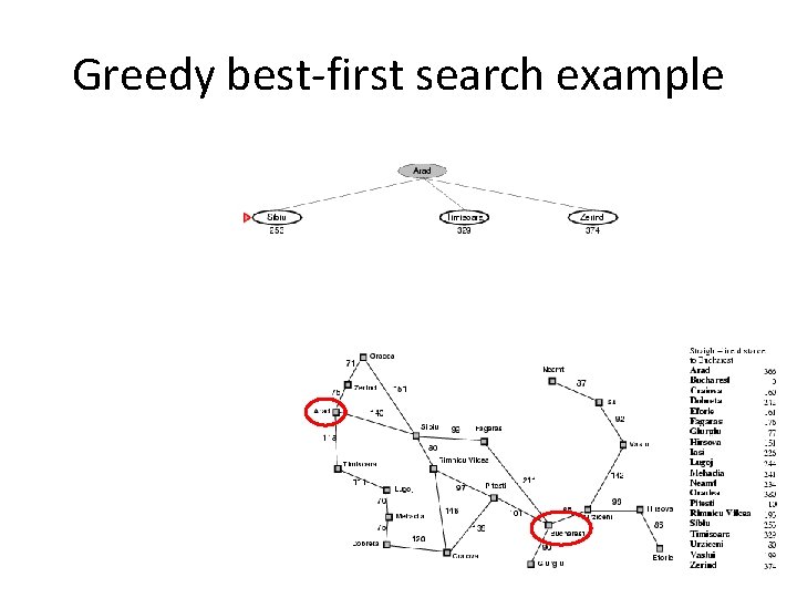
Greedy best-first search example
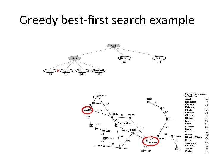
Greedy best-first search example
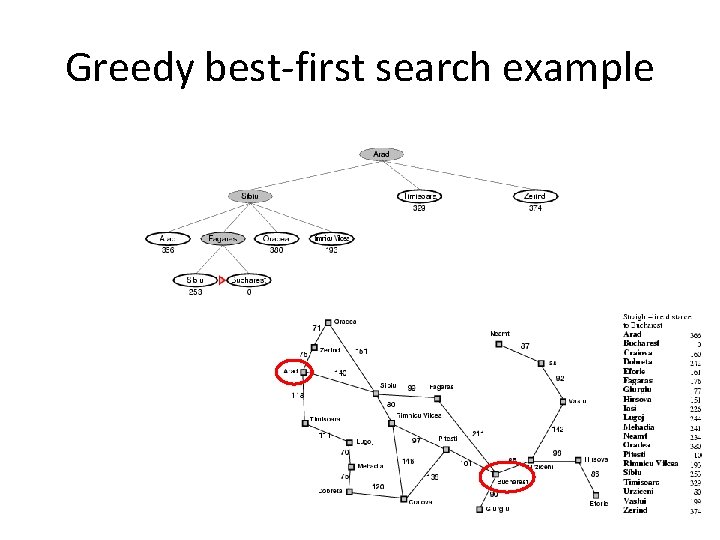
Greedy best-first search example
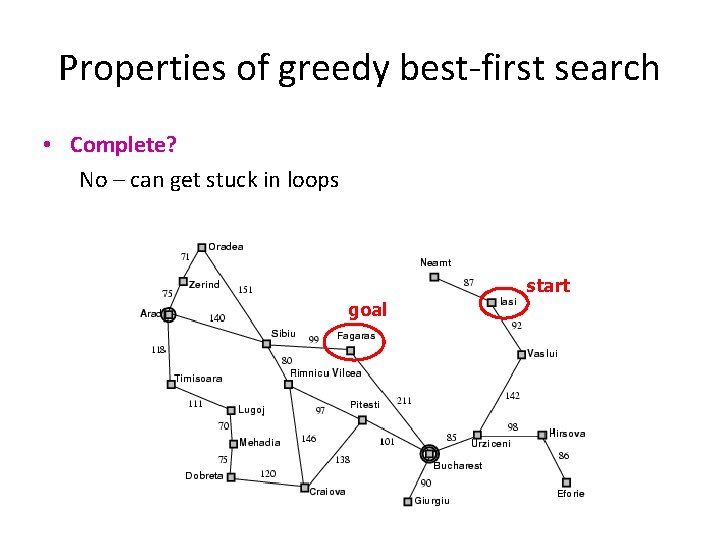
Properties of greedy best-first search • Complete? No – can get stuck in loops start goal
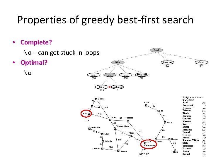
Properties of greedy best-first search • Complete? No – can get stuck in loops • Optimal? No
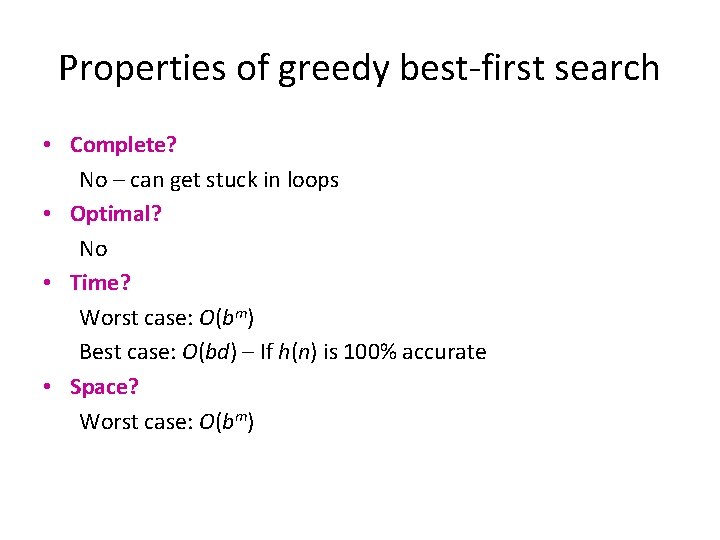
Properties of greedy best-first search • Complete? No – can get stuck in loops • Optimal? No • Time? Worst case: O(bm) Best case: O(bd) – If h(n) is 100% accurate • Space? Worst case: O(bm)
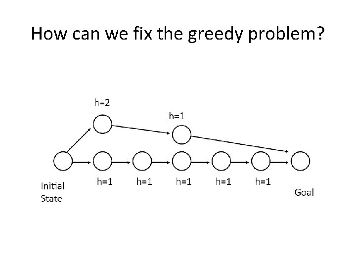
How can we fix the greedy problem?
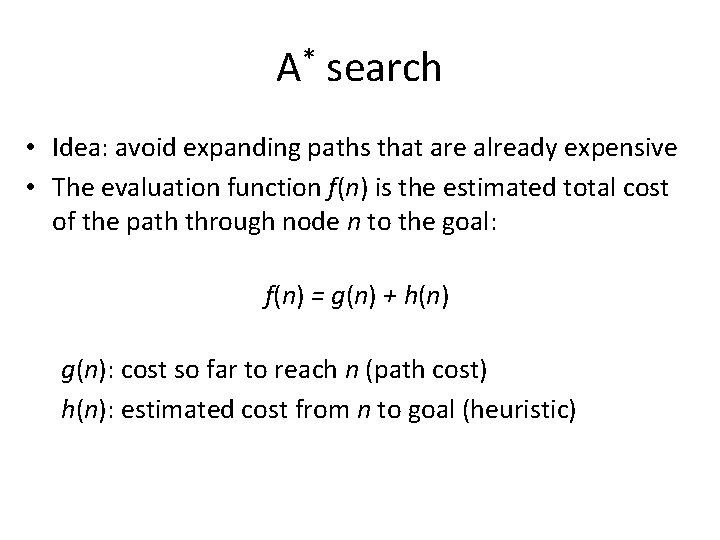
A* search • Idea: avoid expanding paths that are already expensive • The evaluation function f(n) is the estimated total cost of the path through node n to the goal: f(n) = g(n) + h(n) g(n): cost so far to reach n (path cost) h(n): estimated cost from n to goal (heuristic)
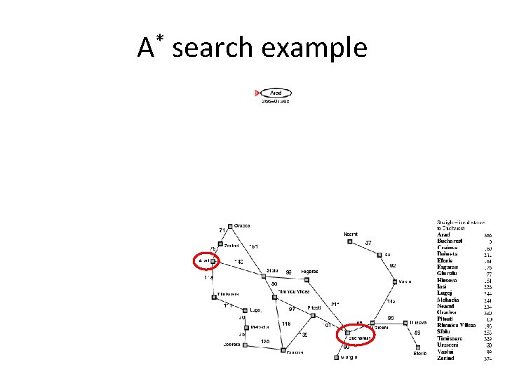
A* search example
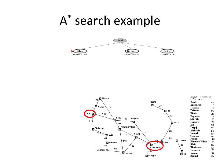
A* search example
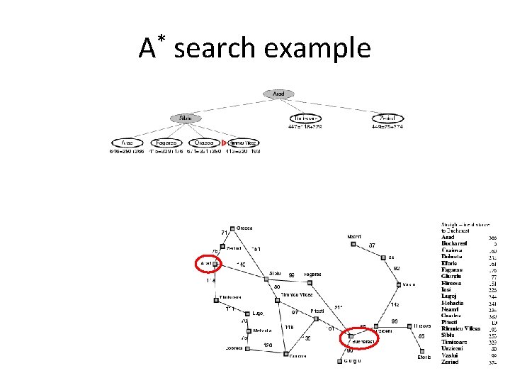
A* search example
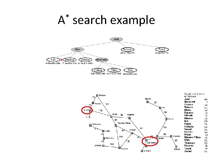
A* search example
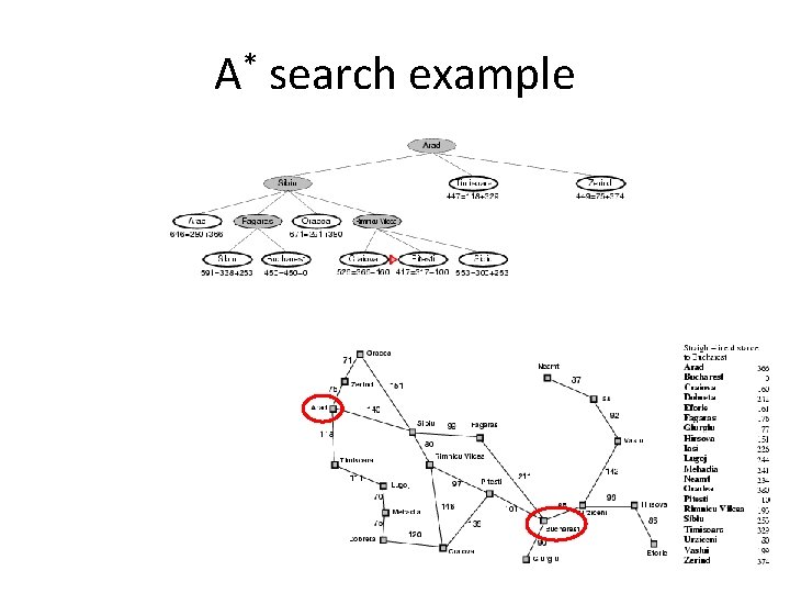
A* search example
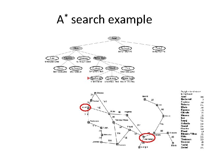
A* search example
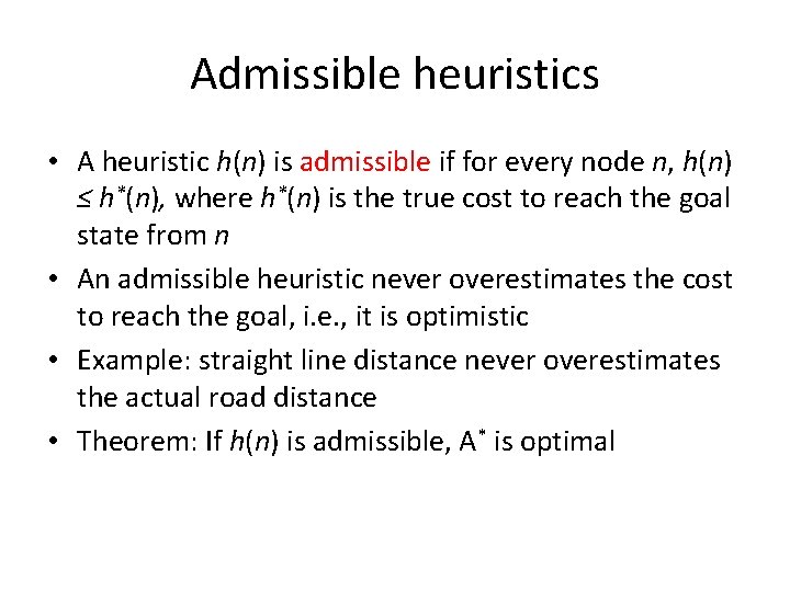
Admissible heuristics • A heuristic h(n) is admissible if for every node n, h(n) ≤ h*(n), where h*(n) is the true cost to reach the goal state from n • An admissible heuristic never overestimates the cost to reach the goal, i. e. , it is optimistic • Example: straight line distance never overestimates the actual road distance • Theorem: If h(n) is admissible, A* is optimal

Optimality of A* n' n* n • Proof by contradiction – Let n* be an optimal goal state, i. e. , f(n*) = C* – Suppose a solution node n with f(n) > C* is about to be expanded – Let n' be a node in the fringe that is on the path to n* – We have f(n') = g(n') + h(n') ≤ C* – But then, n' should be expanded before n – a contradiction
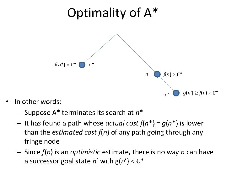
Optimality of A* f(n*) = C* n* n f(n) > C* n' g(n') f(n) > C* • In other words: – Suppose A* terminates its search at n* – It has found a path whose actual cost f(n*) = g(n*) is lower than the estimated cost f(n) of any path going through any fringe node – Since f(n) is an optimistic estimate, there is no way n can have a successor goal state n’ with g(n’) < C*
Optimality of A* • A* is optimally efficient – no other tree-based algorithm that uses the same heuristic can expand fewer nodes and still be guaranteed to find the optimal solution – Any algorithm that does not expand all nodes with f(n) < C* risks missing the optimal solution
Properties of A* • Complete? Yes – unless there are infinitely many nodes with f(n) ≤ C* • Optimal? Yes • Time? Number of nodes for which f(n) ≤ C* (exponential) • Space? Exponential
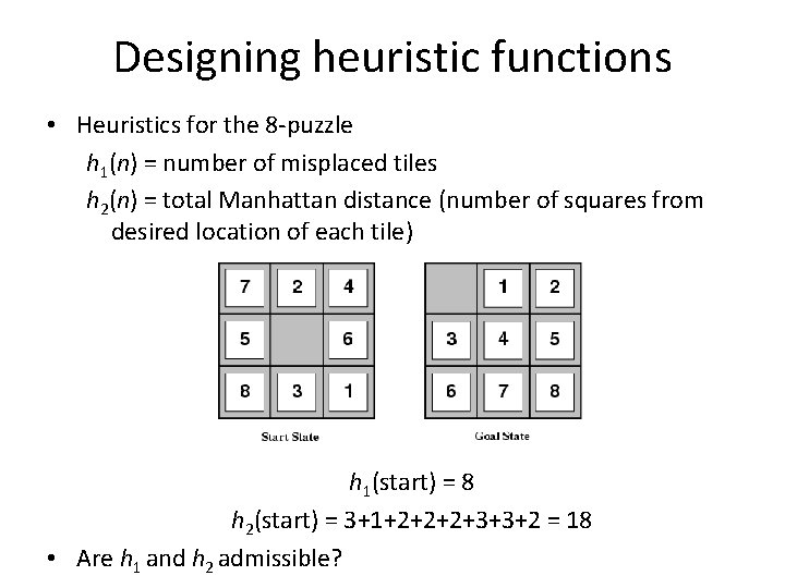
Designing heuristic functions • Heuristics for the 8 -puzzle h 1(n) = number of misplaced tiles h 2(n) = total Manhattan distance (number of squares from desired location of each tile) h 1(start) = 8 h 2(start) = 3+1+2+2+2+3+3+2 = 18 • Are h 1 and h 2 admissible?
Heuristics from relaxed problems • A problem with fewer restrictions on the actions is called a relaxed problem • The cost of an optimal solution to a relaxed problem is an admissible heuristic for the original problem • If the rules of the 8 -puzzle are relaxed so that a tile can move anywhere, then h 1(n) gives the shortest solution • If the rules are relaxed so that a tile can move to any adjacent square, then h 2(n) gives the shortest solution
Dominance • If h 1 and h 2 are both admissible heuristics and h 2(n) ≥ h 1(n) for all n, (both admissible) then h 2 dominates h 1 • Which one is better for search? – A* search expands every node with f(n) < C* or h(n) < C* – g(n) – Therefore, A* search with h 1 will expand more nodes
Dominance • Typical search costs for the 8 -puzzle (average number of nodes expanded for different solution depths): • d=12 IDS = 3, 644, 035 nodes A*(h 1) = 227 nodes A*(h 2) = 73 nodes • d=24 IDS ≈ 54, 000, 000 nodes A*(h 1) = 39, 135 nodes A*(h 2) = 1, 641 nodes
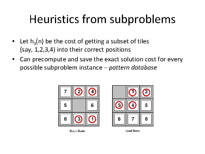
Heuristics from subproblems • Let h 3(n) be the cost of getting a subset of tiles (say, 1, 2, 3, 4) into their correct positions • Can precompute and save the exact solution cost for every possible subproblem instance – pattern database
Combining heuristics • Suppose we have a collection of admissible heuristics h 1(n), h 2(n), …, hm(n), but none of them dominates the others • How can we combine them? h(n) = max{h 1(n), h 2(n), …, hm(n)}
Memory-bounded search • The memory usage of A* can still be exorbitant • How to make A* more memory-efficient while maintaining completeness and optimality? • Iterative deepening A* search • Recursive best-first search, SMA* – Forget some subtrees but remember the best f-value in these subtrees and regenerate them later if necessary • Problems: memory-bounded strategies can be complicated to implement, suffer from “thrashing”
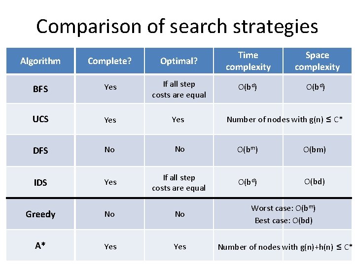
Comparison of search strategies Algorithm Complete? Optimal? Time complexity Space complexity BFS Yes If all step costs are equal O(bd) UCS Yes DFS No No O(bm) IDS Yes If all step costs are equal O(bd) Number of nodes with g(n) ≤ C* Greedy No No Worst case: O(bm) Best case: O(bd) A* Yes Number of nodes with g(n)+h(n) ≤ C*
- Slides: 59