Review Probability Chapter 13 Basic probability notationdefinitions Probability

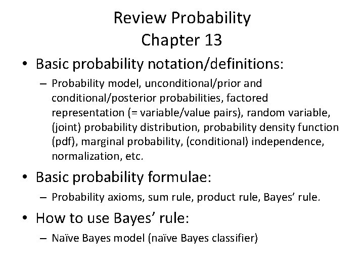
Review Probability Chapter 13 • Basic probability notation/definitions: – Probability model, unconditional/prior and conditional/posterior probabilities, factored representation (= variable/value pairs), random variable, (joint) probability distribution, probability density function (pdf), marginal probability, (conditional) independence, normalization, etc. • Basic probability formulae: – Probability axioms, sum rule, product rule, Bayes’ rule. • How to use Bayes’ rule: – Naïve Bayes model (naïve Bayes classifier)

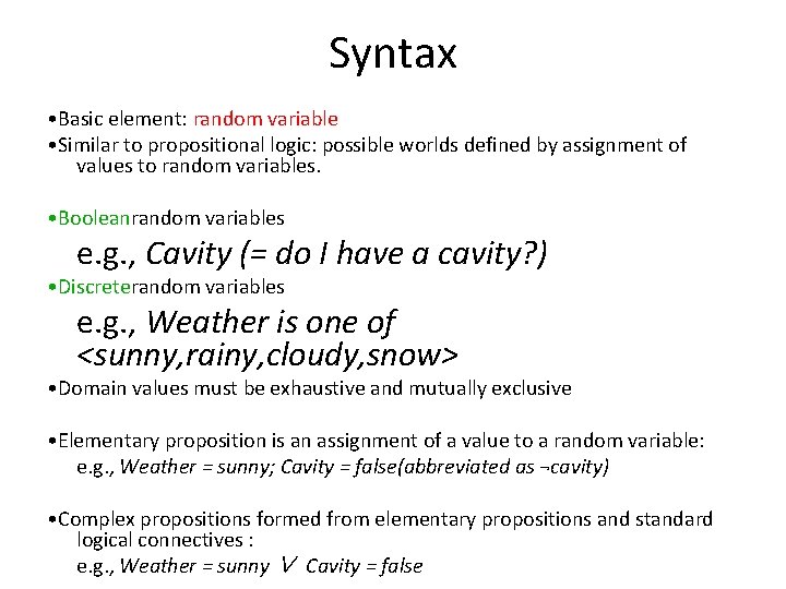
Syntax • Basic element: random variable • Similar to propositional logic: possible worlds defined by assignment of values to random variables. • Booleanrandom variables e. g. , Cavity (= do I have a cavity? ) • Discreterandom variables e. g. , Weather is one of <sunny, rainy, cloudy, snow> • Domain values must be exhaustive and mutually exclusive • Elementary proposition is an assignment of a value to a random variable: e. g. , Weather = sunny; Cavity = false(abbreviated as ¬cavity) • Complex propositions formed from elementary propositions and standard logical connectives : e. g. , Weather = sunny ∨ Cavity = false

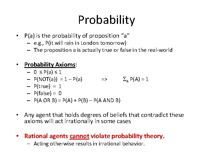
Probability • P(a) is the probability of proposition “a” – e. g. , P(it will rain in London tomorrow) – The proposition a is actually true or false in the real-world • Probability Axioms: – – – 0 ≤ P(a) ≤ 1 P(NOT(a)) = 1 – P(a) => A P(A) = 1 P(true) = 1 P(false) = 0 P(A OR B) = P(A) + P(B) – P(A AND B) • Any agent that holds degrees of beliefs that contradict these axioms will act irrationally in some cases • Rational agents cannot violate probability theory. ─ Acting otherwise results in irrational behavior.

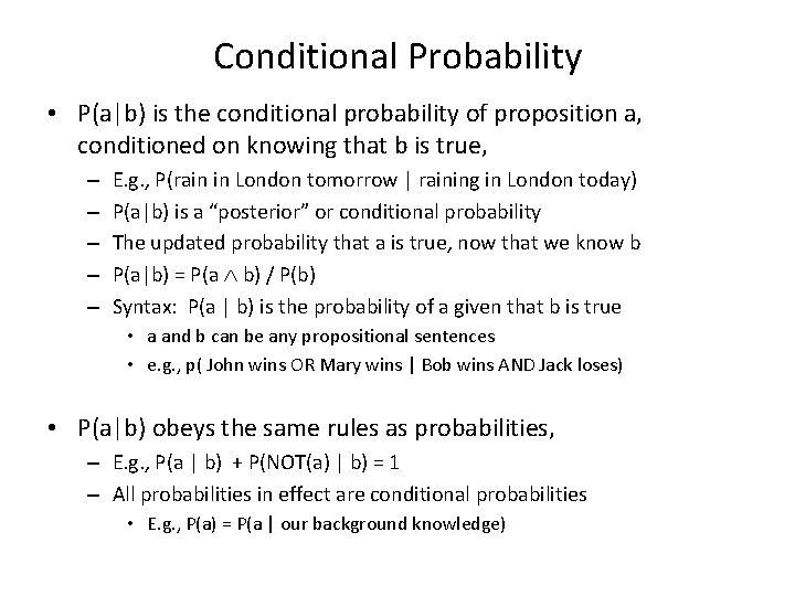
Conditional Probability • P(a|b) is the conditional probability of proposition a, conditioned on knowing that b is true, – – – E. g. , P(rain in London tomorrow | raining in London today) P(a|b) is a “posterior” or conditional probability The updated probability that a is true, now that we know b P(a|b) = P(a b) / P(b) Syntax: P(a | b) is the probability of a given that b is true • a and b can be any propositional sentences • e. g. , p( John wins OR Mary wins | Bob wins AND Jack loses) • P(a|b) obeys the same rules as probabilities, – E. g. , P(a | b) + P(NOT(a) | b) = 1 – All probabilities in effect are conditional probabilities • E. g. , P(a) = P(a | our background knowledge)

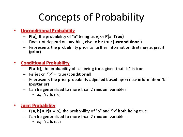
Concepts of Probability • Unconditional Probability ─ P(a), the probability of “a” being true, or P(a=True) ─ Does not depend on anything else to be true (unconditional) ─ Represents the probability prior to further information that may adjust it (prior) • Conditional Probability ─ P(a|b), the probability of “a” being true, given that “b” is true ─ Relies on “b” = true (conditional) ─ Represents the prior probability adjusted based upon new information “b” (posterior) ─ Can be generalized to more than 2 random variables: § e. g. P(a|b, c, d) • Joint Probability ─ P(a, b) = P(a ˄ b), the probability of “a” and “b” both being true ─ Can be generalized to more than 2 random variables: § e. g. P(a, b, c, d)

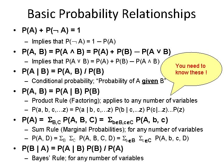
Basic Probability Relationships • P(A) + P( A) = 1 – Implies that P( A) = 1 ─ P(A) • P(A, B) = P(A ˄ B) = P(A) + P(B) ─ P(A ˅ B) – Implies that P(A ˅ B) = P(A) + P(B) ─ P(A ˄ B) • P(A | B) = P(A, B) / P(B) You need to know these ! – Conditional probability; “Probability of A given B” • P(A, B) = P(A | B) P(B) – Product Rule (Factoring); applies to any number of variables – P(a, b, c, …z) = P(a | b, c, …z) P(b | c, . . . z) P(c|. . . z). . . P(z) • P(A) = B, C P(A, B, C) = b B, c C P(A, b, c) – Sum Rule (Marginal Probabilities); for any number of variables – P(A, D) = B C P(A, B, C, D) = b B c C P(A, b, c, D) • P(B | A) = P(A | B) P(B) / P(A) – Bayes’ Rule; for any number of variables

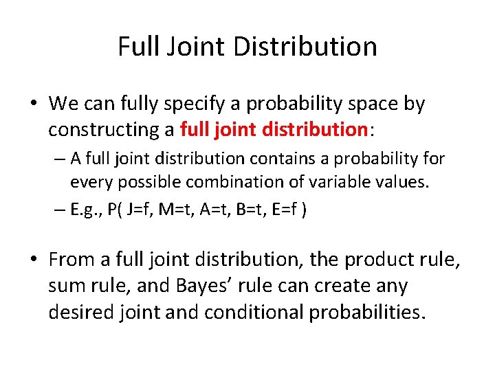
Full Joint Distribution • We can fully specify a probability space by constructing a full joint distribution: – A full joint distribution contains a probability for every possible combination of variable values. – E. g. , P( J=f, M=t, A=t, B=t, E=f ) • From a full joint distribution, the product rule, sum rule, and Bayes’ rule can create any desired joint and conditional probabilities.

Computing with Probabilities: Law of Total Probability (aka “summing out” or marginalization) P(a) = b P(a, b) = b P(a | b) P(b) where B is any random variable Why is this useful? Given a joint distribution (e. g. , P(a, b, c, d)) we can obtain any “marginal” probability (e. g. , P(b)) by summing out the other variables, e. g. , P(b) = a c d P(a, b, c, d) We can compute any conditional probability given a joint distribution, e. g. , P(c | b) = a d P(a, c, d, b) / P(b) where P(b) can be computed as above

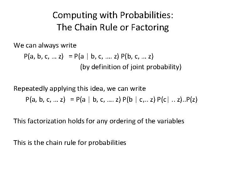
Computing with Probabilities: The Chain Rule or Factoring We can always write P(a, b, c, … z) = P(a | b, c, …. z) P(b, c, … z) (by definition of joint probability) Repeatedly applying this idea, we can write P(a, b, c, … z) = P(a | b, c, …. z) P(b | c, . . z) P(c|. . z). . P(z) This factorization holds for any ordering of the variables This is the chain rule for probabilities

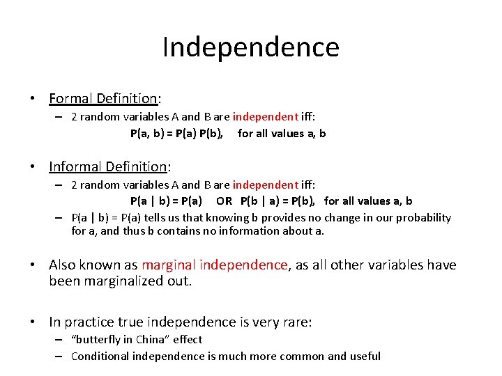
Independence • Formal Definition: – 2 random variables A and B are independent iff: P(a, b) = P(a) P(b), for all values a, b • Informal Definition: – 2 random variables A and B are independent iff: P(a | b) = P(a) OR P(b | a) = P(b), for all values a, b – P(a | b) = P(a) tells us that knowing b provides no change in our probability for a, and thus b contains no information about a. • Also known as marginal independence, as all other variables have been marginalized out. • In practice true independence is very rare: – “butterfly in China” effect – Conditional independence is much more common and useful

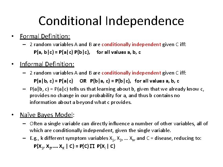
Conditional Independence • Formal Definition: – 2 random variables A and B are conditionally independent given C iff: P(a, b|c) = P(a|c) P(b|c), for all values a, b, c • Informal Definition: – 2 random variables A and B are conditionally independent given C iff: P(a|b, c) = P(a|c) OR P(b|a, c) = P(b|c), for all values a, b, c – P(a|b, c) = P(a|c) tells us that learning about b, given that we already know c, provides no change in our probability for a, and thus b contains no information about a beyond what c provides. • Naïve Bayes Model: – Often a single variable can directly influence a number of other variables, all of which are conditionally independent, given the single variable. – E. g. , k different symptom variables X 1, X 2, … Xk, and C = disease, reducing to: P(X 1, X 2, …. XK | C) = P(C) P P(Xi | C)

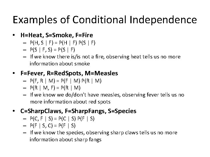
Examples of Conditional Independence • H=Heat, S=Smoke, F=Fire – P(H, S | F) = P(H | F) P(S | F) – P(S | F, S) = P(S | F) – If we know there is/is not a fire, observing heat tells us no more information about smoke • F=Fever, R=Red. Spots, M=Measles – P(F, R | M) = P(F | M) P(R | M) – P(R | M, F) = P(R | M) – If we know we do/don’t have measles, observing fever tells us no more information about red spots • C=Sharp. Claws, F=Sharp. Fangs, S=Species – P(C, F | S) = P(C | S) P(F | S) – P(F | S, C) = P(F | S) – If we know the species, observing sharp claws tells us no more information about sharp fangs