Review Part 1 CSE 2011 Winter 2011 1022020

Review – Part 1 CSE 2011 Winter 2011 10/2/2020 1

Algorithm Analysis l Given an algorithm, compute its running time in terms of O, , and (if any). ¡ Usually the big-Oh running time is enough. l Given f(n) = 5 n + 10, show that f(n) is O(n). ¡ Find c and n 0 l Compare the grow rates of 2 functions. l Order the grow rates of several functions. ¡ Use slide 14. ¡ Use L’Hôpital’s rule. 2

Running Times of Loops Nested for loops: l If the exact number of iterations of each loop is known, multiply the numbers of iterations of the loops. l If the exact number of iterations of some loop is not known, “open” the loops and count the total number of iterations. 3

Running Time of Recursive Methods l Could be just a hidden “for" or “while” loop. ¡See “Tail Recursion” slide. ¡“Unravel” the hidden loop to count the number of iterations. l Logarithmic ¡Examples: binary search, exponentiation, GCD l Solving a recurrence ¡Example: merge sort, quick sort 4

Recursion Know how to write recursive functions/methods: l Recursive call ¡ Adjusting recursive parameter(s) for each call l Base case(s) 1. Use the definition (factorial, tree depth, height) 2. Cut the problem size by half (binary search), or by k elements at a time (sum, reversing arrays). 3. Divide and conquer (merge sort, quick sort) 5

Sorting Algorithms l Insertion sort l Merge sort l Quick sort l Lower bound of sorting algorithms ¡O(Nlog. N) l When to use which sorting algorithm? l Linear-time sorting (bucket sort) 6

Running Time of Tree Methods Most tree methods are recursive. l Visualize the recursion trace. l Count the number of nodes that were visited (processed) k. l Compute the running time for processing each node O(m). l If O(mv) ≠ O(mu), sum up the running times of the k nodes. l Otherwise total running time = k O(m) 7

Arrays and Linked Lists Arrays l A = B l Cloning arrays l Extendable arrays l Strategies for extending arrays: ¡doubling the size ¡increment by k cells Linked lists l Singly linked l Doubly linked l Implementation l Running times for insertion and deletion at the two ends. 8

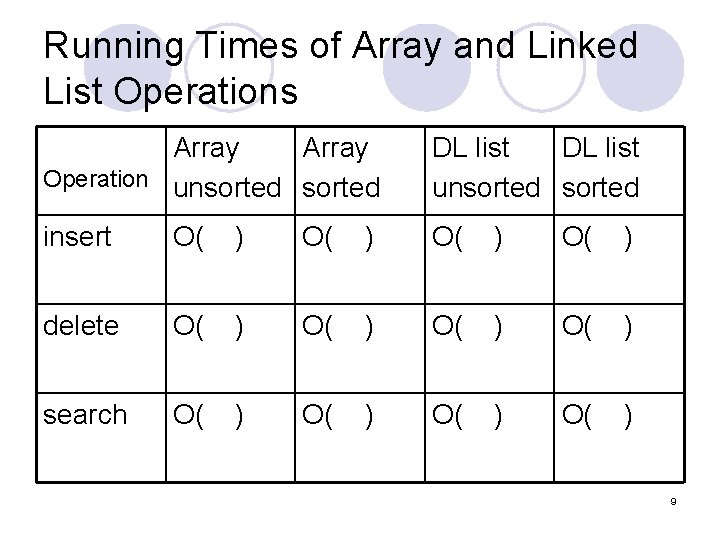
Running Times of Array and Linked List Operations Array Operation unsorted DL list unsorted insert O( ) delete O( ) search O( ) 9

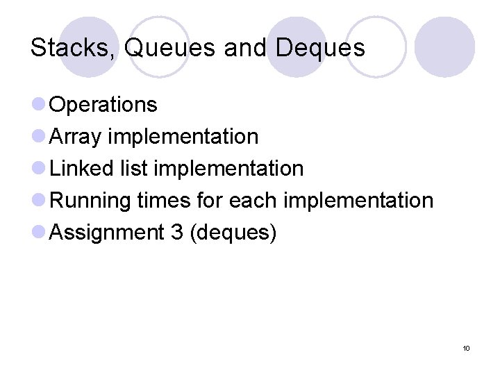
Stacks, Queues and Deques l Operations l Array implementation l Linked list implementation l Running times for each implementation l Assignment 3 (deques) 10

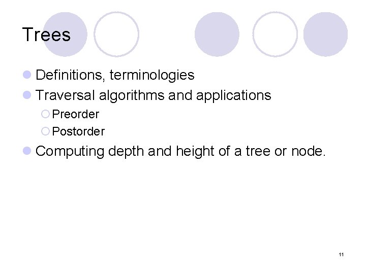
Trees l Definitions, terminologies l Traversal algorithms and applications ¡Preorder ¡Postorder l Computing depth and height of a tree or node. 11

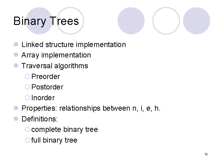
Binary Trees l Linked structure implementation l Array implementation l Traversal algorithms ¡Preorder ¡Postorder ¡Inorder l Properties: relationships between n, i, e, h. l Definitions: ¡complete binary tree ¡full binary tree 12

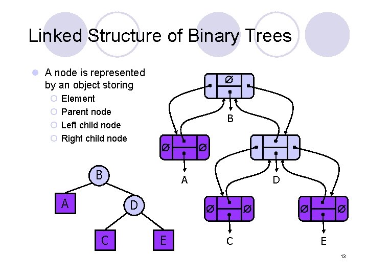
Linked Structure of Binary Trees l A node is represented by an object storing ¡ ¡ Element Parent node Left child node Right child node B B A A D C D E C E 13

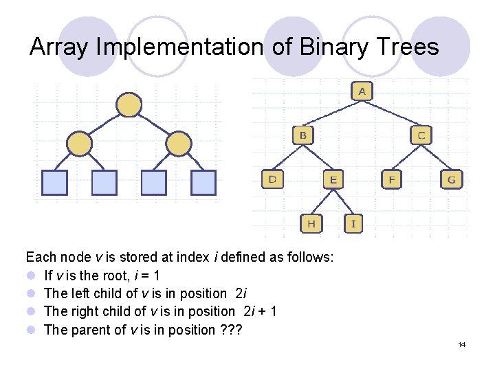
Array Implementation of Binary Trees Each node v is stored at index i defined as follows: l If v is the root, i = 1 l The left child of v is in position 2 i l The right child of v is in position 2 i + 1 l The parent of v is in position ? ? ? 14

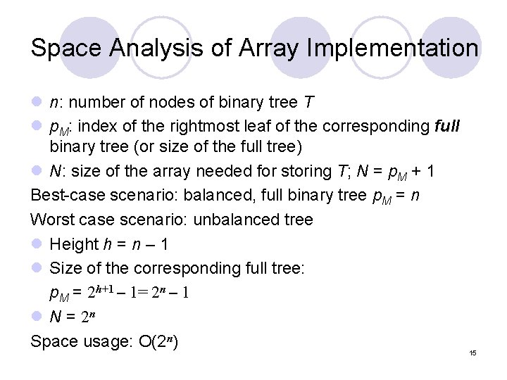
Space Analysis of Array Implementation l n: number of nodes of binary tree T l p. M: index of the rightmost leaf of the corresponding full binary tree (or size of the full tree) l N: size of the array needed for storing T; N = p. M + 1 Best-case scenario: balanced, full binary tree p. M = n Worst case scenario: unbalanced tree l Height h = n – 1 l Size of the corresponding full tree: p. M = 2 h+1 – 1= 2 n – 1 l N = 2 n Space usage: O(2 n) 15

Arrays versus Linked Structure Linked lists l Slower operations due to pointer manipulations l Use less space if the tree is unbalanced l Rotation (restructuring) code is simple Arrays l Faster operations l Use less space if the tree is balanced (no pointers) l Rotation (restructuring) code is complex 16

Review – Part 2 CSE 2011 10/2/2020 17

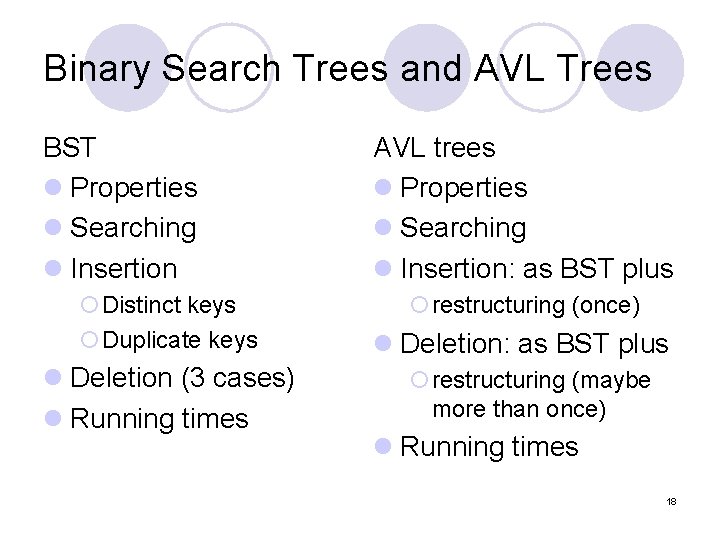
Binary Search Trees and AVL Trees BST l Properties l Searching l Insertion ¡Distinct keys ¡Duplicate keys l Deletion (3 cases) l Running times AVL trees l Properties l Searching l Insertion: as BST plus ¡restructuring (once) l Deletion: as BST plus ¡restructuring (maybe more than once) l Running times 18

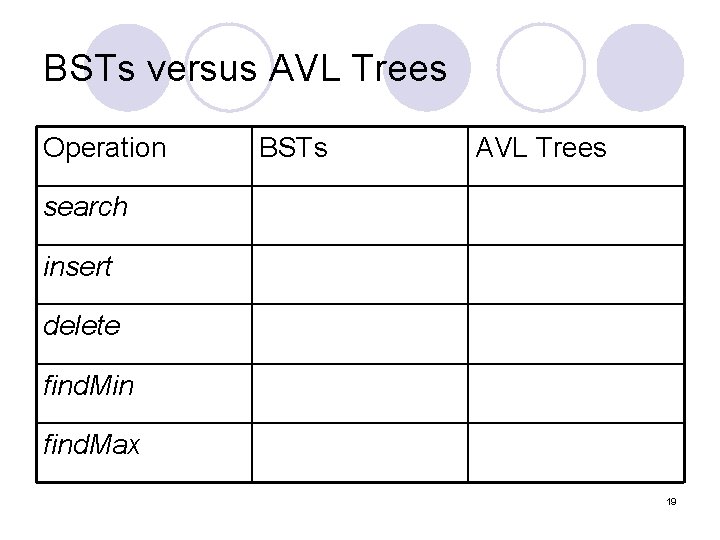
BSTs versus AVL Trees Operation BSTs AVL Trees search insert delete find. Min find. Max 19

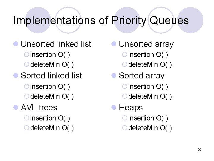
Implementations of Priority Queues l Unsorted linked list ¡ insertion O( ) ¡ delete. Min O( ) l Sorted linked list ¡ insertion O( ) ¡ delete. Min O( ) l AVL trees ¡ insertion O( ) ¡ delete. Min O( ) l Unsorted array ¡ insertion O( ) ¡ delete. Min O( ) l Sorted array ¡ insertion O( ) ¡ delete. Min O( ) l Heaps ¡ insertion O( ) ¡ delete. Min O( ) 20

Heaps l Properties l Array implementation l Insert ¡upheap percolation l Other operations: ¡decrease. Key(i, k) ¡increase. Key(i, k) ¡delete(i) l Delete ¡downheap percolation l Running time 21

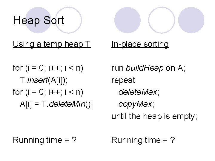
Heap Sort Using a temp heap T In-place sorting for (i = 0; i++; i < n) T. insert(A[i]); for (i = 0; i++; i < n) A[i] = T. delete. Min(); run build. Heap on A; repeat delete. Max; copy. Max; until the heap is empty; Running time = ?

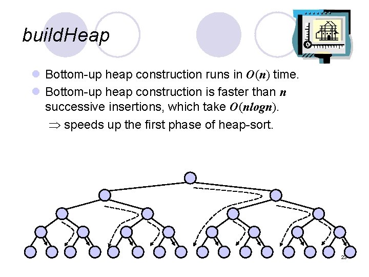
build. Heap l Bottom-up heap construction runs in O(n) time. l Bottom-up heap construction is faster than n successive insertions, which take O(nlogn). speeds up the first phase of heap-sort. 23

Hashing l Table size (a prime number) l Hash functions ¡ For integer keys l division (modular) l MAD ¡ For strings: polynomial accumulation Collision handling l Separate chaining l Probing (open addressing) ¡Linear probing ¡Quadratic probing ¡Double hashing l z = 33, 37, 39, 41 l Probing: 3 types of cells (null, in use, available) 24

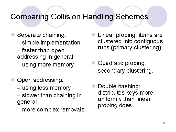
Comparing Collision Handling Schemes l Separate chaining: – simplementation – faster than open addressing in general – using more memory l Linear probing: items are clustered into contiguous runs (primary clustering). l Quadratic probing: secondary clustering. l Open addressing: l Double hashing: – using less memory distributes keys more – slower than chaining in uniformly than linear general probing does. – more complex removals 25

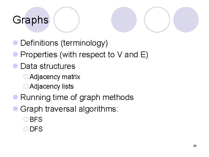
Graphs l Definitions (terminology) l Properties (with respect to V and E) l Data structures ¡ Adjacency matrix ¡ Adjacency lists l Running time of graph methods l Graph traversal algorithms: ¡ BFS ¡ DFS 26

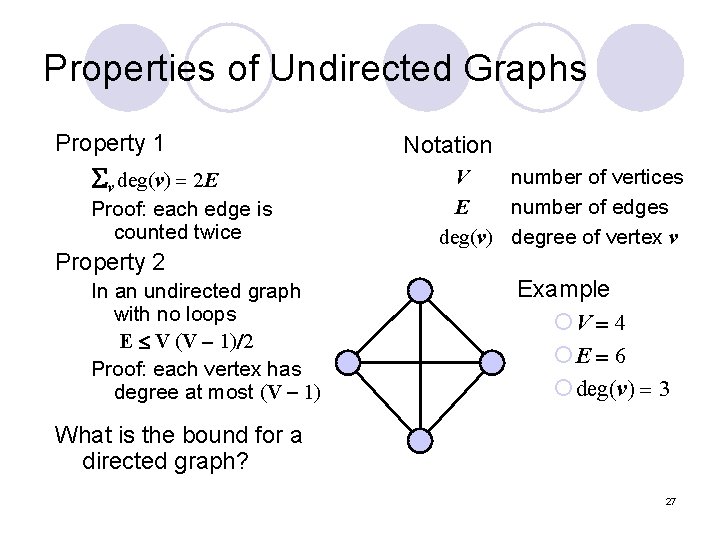
Properties of Undirected Graphs Property 1 Sv deg(v) = 2 E Proof: each edge is counted twice Property 2 In an undirected graph with no loops E V (V - 1)/2 Proof: each vertex has degree at most (V - 1) Notation V number of vertices E number of edges deg(v) degree of vertex v Example ¡V = 4 ¡E = 6 ¡ deg(v) = 3 What is the bound for a directed graph? 27

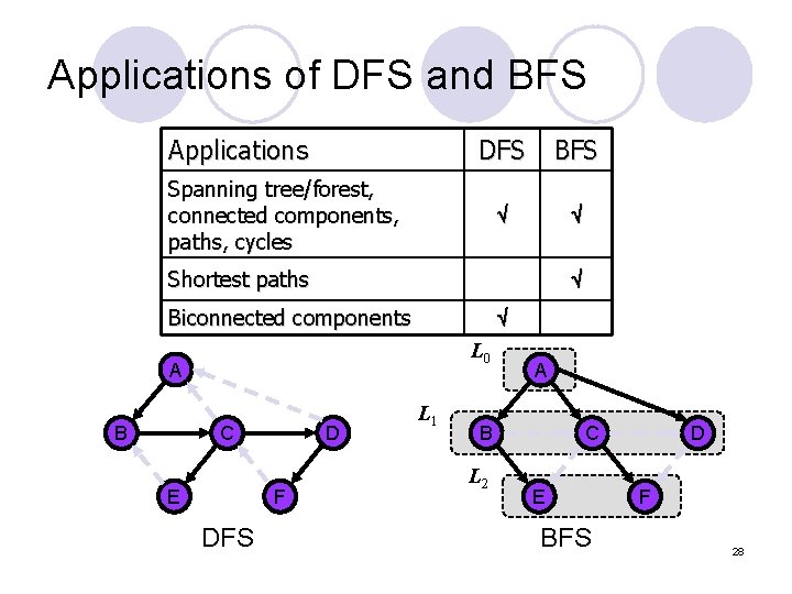
Applications of DFS and BFS Applications DFS BFS Spanning tree/forest, connected components, paths, cycles Shortest paths Biconnected components L 0 A B C E D F DFS L 1 A B L 2 C E BFS D F 28

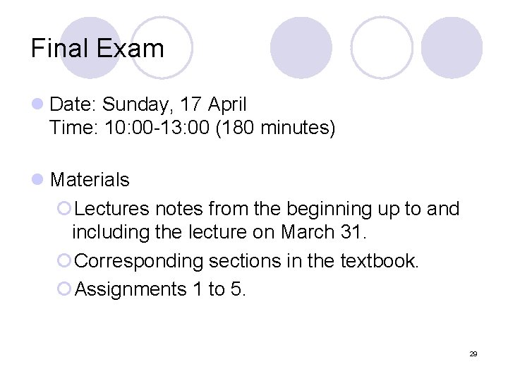
Final Exam l Date: Sunday, 17 April Time: 10: 00 -13: 00 (180 minutes) l Materials ¡Lectures notes from the beginning up to and including the lecture on March 31. ¡Corresponding sections in the textbook. ¡Assignments 1 to 5. 29

Exam Rules l This is a closed-book exam. No books, notes or calculators are allowed. You will be given blank paper for scrap work. l Bring a photo ID, pens, and pencils. You may use pencils with darkness of at least HB; 2 B is preferred. l No questions are allowed during the exam. l You may leave the classroom if you hand in your exam booklet 10 minutes or more before the exam ends. 30 l

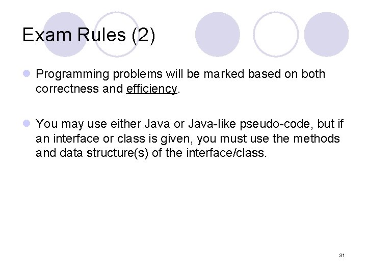
Exam Rules (2) l Programming problems will be marked based on both correctness and efficiency. l You may use either Java or Java-like pseudo-code, but if an interface or class is given, you must use the methods and data structure(s) of the interface/class. 31

Office Hours before Exam (tentative) l Wednesday, 6 April, 11: 00 -12: 00 l Thursday, 14 April, 14: 00 -15: 00 32