Review of Probability Axioms of Probability Theory PrA

Review of Probability

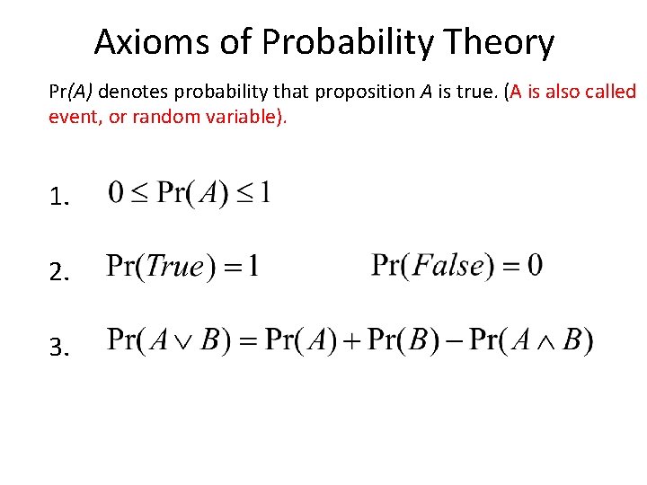
Axioms of Probability Theory Pr(A) denotes probability that proposition A is true. (A is also called event, or random variable). 1. 2. 3.

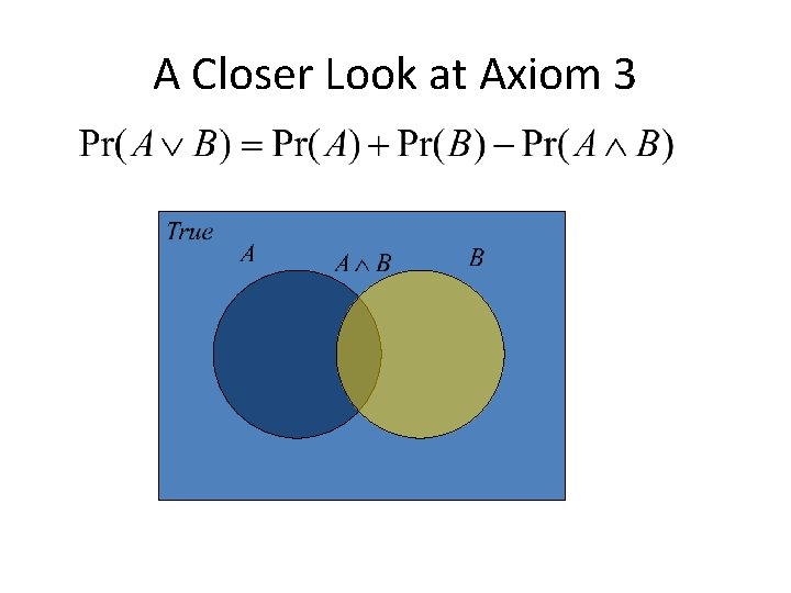
A Closer Look at Axiom 3 B

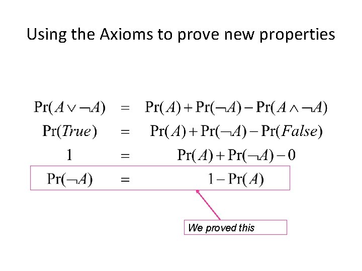
Using the Axioms to prove new properties We proved this

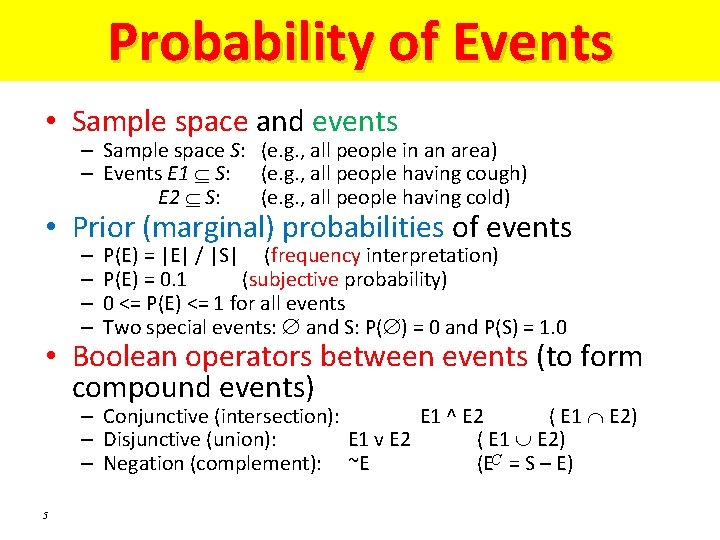
Probability of Events • Sample space and events – Sample space S: (e. g. , all people in an area) – Events E 1 S: (e. g. , all people having cough) E 2 S: (e. g. , all people having cold) • Prior (marginal) probabilities of events – – P(E) = |E| / |S| (frequency interpretation) P(E) = 0. 1 (subjective probability) 0 <= P(E) <= 1 for all events Two special events: and S: P( ) = 0 and P(S) = 1. 0 • Boolean operators between events (to form compound events) – Conjunctive (intersection): E 1 ^ E 2 ( E 1 E 2) – Disjunctive (union): E 1 v E 2 ( E 1 E 2) – Negation (complement): ~E (EC = S – E) 5

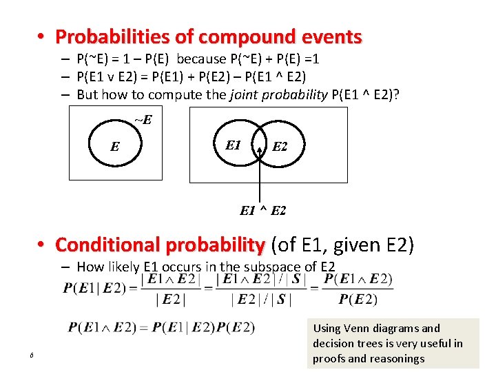
• Probabilities of compound events – P(~E) = 1 – P(E) because P(~E) + P(E) =1 – P(E 1 v E 2) = P(E 1) + P(E 2) – P(E 1 ^ E 2) – But how to compute the joint probability P(E 1 ^ E 2)? ~E E E 1 E 2 E 1 ^ E 2 • Conditional probability (of E 1, given E 2) – How likely E 1 occurs in the subspace of E 2 6 Using Venn diagrams and decision trees is very useful in proofs and reasonings

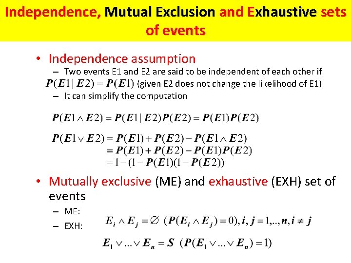
Independence, Mutual Exclusion and Exhaustive sets of events • Independence assumption – Two events E 1 and E 2 are said to be independent of each other if (given E 2 does not change the likelihood of E 1) – It can simplify the computation • Mutually exclusive (ME) and exhaustive (EXH) set of events – ME: – EXH:

Random Variables 8

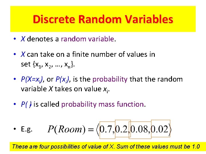
Discrete Random Variables • X denotes a random variable. • X can take on a finite number of values in set {x 1, x 2, …, xn}. • P(X=xi), or P(xi), is the probability that the random variable X takes on value xi. • P( ). is called probability mass function. • E. g. These are four possibilities of value of X. Sum of these values must be 1. 0

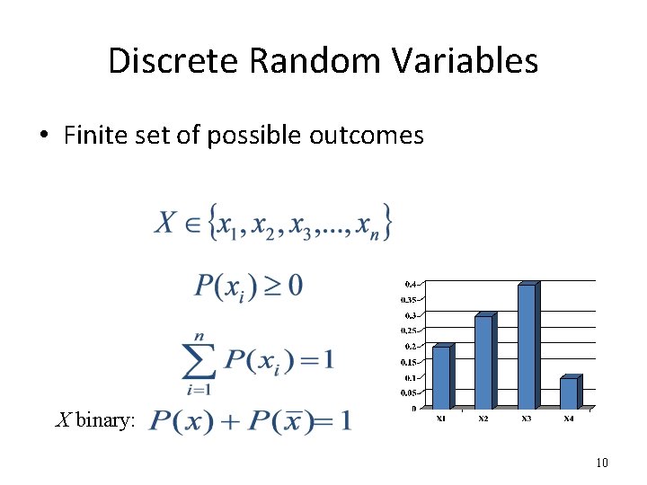
Discrete Random Variables • Finite set of possible outcomes X binary: 10

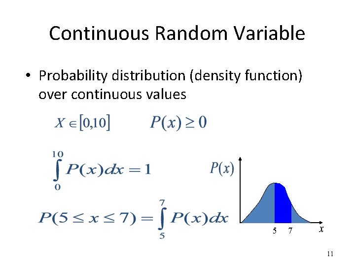
Continuous Random Variable • Probability distribution (density function) over continuous values 5 7 11

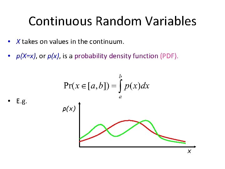
Continuous Random Variables • X takes on values in the continuum. • p(X=x), or p(x), is a probability density function (PDF). • E. g. p(x) x

Probability Distribution • Probability distribution P(X|x) – X is a random variable • Discrete • Continuous – x is background state of information

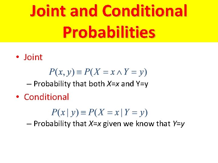
Joint and Conditional Probabilities • Joint – Probability that both X=x and Y=y • Conditional – Probability that X=x given we know that Y=y

Joint and Conditional Probabilities • Joint – Probability that both X=x and Y=y • Conditional – Probability that X=x given we know that Y=y

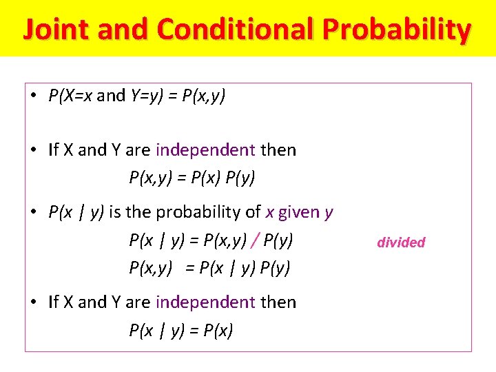
Joint and Conditional Probability • P(X=x and Y=y) = P(x, y) • If X and Y are independent then P(x, y) = P(x) P(y) • P(x | y) is the probability of x given y P(x | y) = P(x, y) / P(y) P(x, y) = P(x | y) P(y) • If X and Y are independent then P(x | y) = P(x) divided

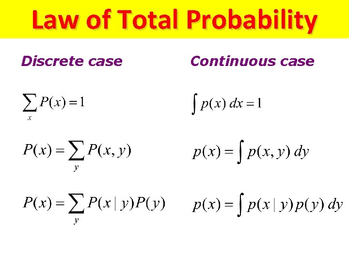
Law of Total Probability Discrete case Continuous case

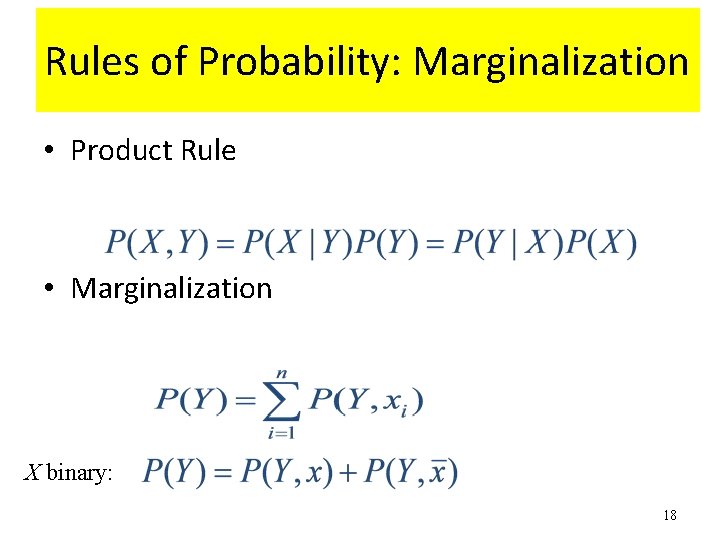
Rules of Probability: Marginalization • Product Rule • Marginalization X binary: 18

Gaussian, Mean and Variance N(m, s)

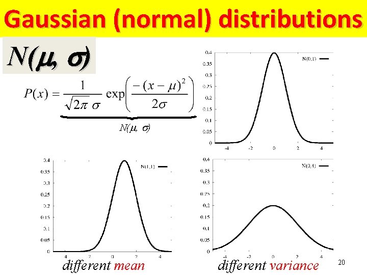
Gaussian (normal) distributions N(m, s) different mean different variance 20

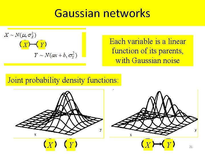
Gaussian networks Each variable is a linear function of its parents, with Gaussian noise Joint probability density functions: X Y 21

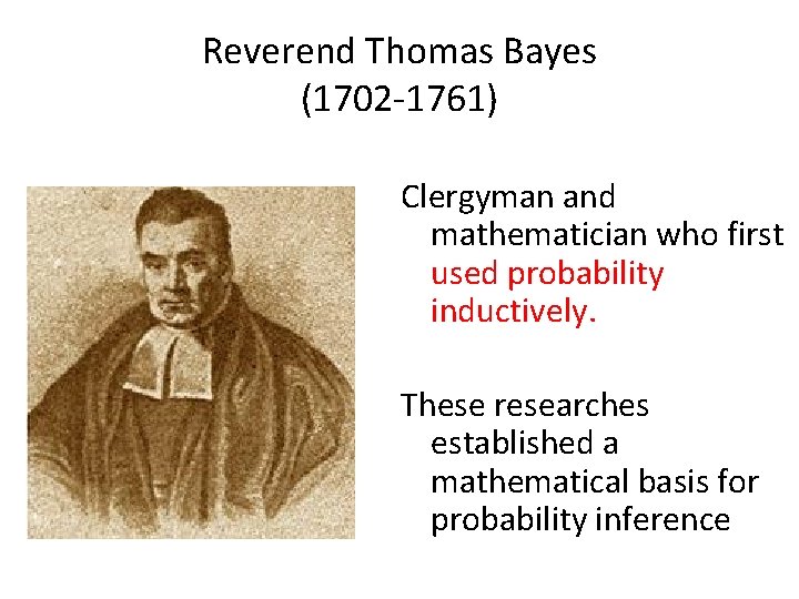
Reverend Thomas Bayes (1702 -1761) Clergyman and mathematician who first used probability inductively. These researches established a mathematical basis for probability inference

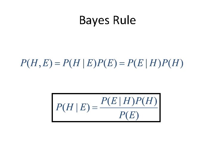
Bayes Rule

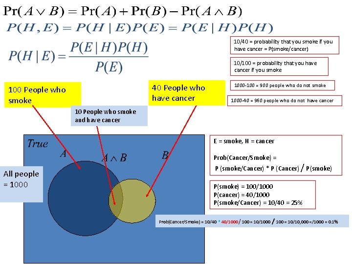
10/40 = probability that you smoke if you have cancer = P(smoke/cancer) 10/100 = probability that you have cancer if you smoke 40 People who have cancer 100 People who smoke 1000 -100 = 900 people who do not smoke 1000 -40 = 960 people who do not have cancer 10 People who smoke and have cancer E = smoke, H = cancer Prob(Cancer/Smoke) = P (smoke/Cancer) * P (Cancer) / P(smoke) All people = 1000 B P(smoke) = 100/1000 P(cancer) = 40/1000 P(smoke/Cancer) = 10/40 = 25% Prob(Cancer/Smoke) = 10/40 * 40/1000 / 100 = 10/10, 000 =/1000 = 0. 1%

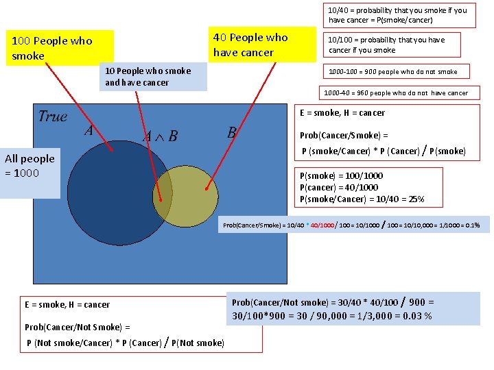
10/40 = probability that you smoke if you have cancer = P(smoke/cancer) 40 People who have cancer 100 People who smoke 10 People who smoke and have cancer 10/100 = probability that you have cancer if you smoke 1000 -100 = 900 people who do not smoke 1000 -40 = 960 people who do not have cancer E = smoke, H = cancer Prob(Cancer/Smoke) = P (smoke/Cancer) * P (Cancer) / P(smoke) All people = 1000 P(smoke) = 100/1000 P(cancer) = 40/1000 P(smoke/Cancer) = 10/40 = 25% B Prob(Cancer/Smoke) = 10/40 * 40/1000 / 100 = 10/10, 000 = 1/1000 = 0. 1% E = smoke, H = cancer Prob(Cancer/Not Smoke) = P (Not smoke/Cancer) * P (Cancer) / P(Not smoke) Prob(Cancer/Not smoke) = 30/40 * 40/100 / 900 = 30/100*900 = 30 / 90, 000 = 1/3, 000 = 0. 03 %

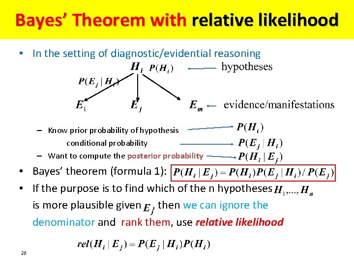
Bayes’ Theorem with relative likelihood • In the setting of diagnostic/evidential reasoning – Know prior probability of hypothesis conditional probability – Want to compute the posterior probability • Bayes’ theorem (formula 1): • If the purpose is to find which of the n hypotheses is more plausible given , then we can ignore the denominator and rank them, use relative likelihood 26

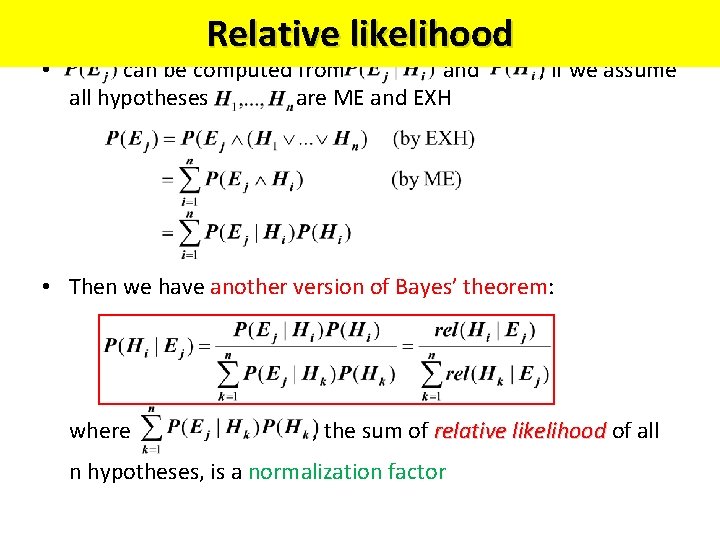
• Relative likelihood can be computed from and all hypotheses are ME and EXH , if we assume • Then we have another version of Bayes’ theorem: where , the sum of relative likelihood of all n hypotheses, is a normalization factor

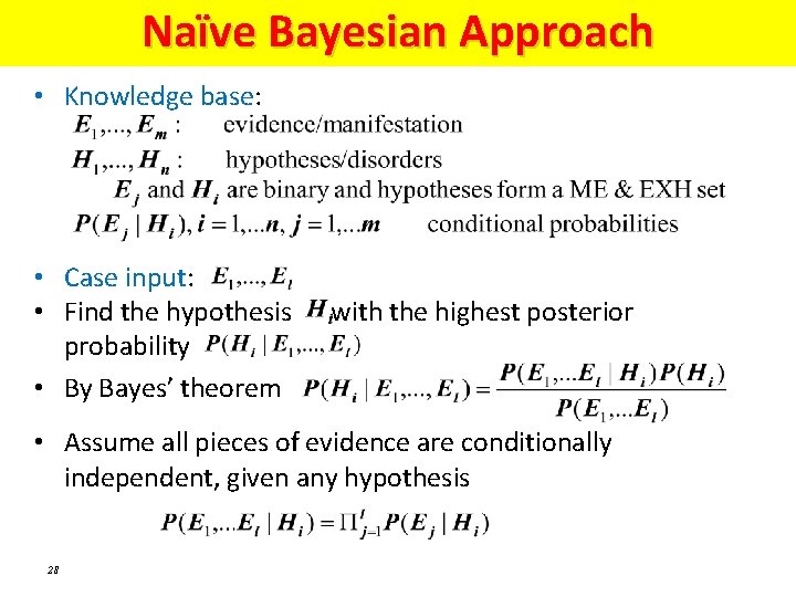
Naïve Bayesian Approach • Knowledge base: • Case input: • Find the hypothesis probability • By Bayes’ theorem with the highest posterior • Assume all pieces of evidence are conditionally independent, given any hypothesis 28

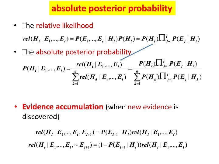
absolute posterior probability • The relative likelihood • The absolute posterior probability • Evidence accumulation (when new evidence is discovered)

Bayesian Networks and Markov Models – applications in robotics • • Bayesian AI Bayesian Filters Kalman Filters Particle Filters Bayesian networks Decision networks Reasoning about changes over time • Dynamic Bayesian Networks • Markov models