Review of Basic Statistical Tools HSE Psychometric School

Review of Basic Statistical Tools. HSE Psychometric School August 2019 Prof. dr. Gavin T. L. Brown University of Auckland Umeå University

Hypotheses Hence, we need to know if our observations are valid… Scientific A suggested solution to a problem; educated, informed, intelligent guess. An empirical proposition testable by experience. Substantive. Important to the real world. I wonder if…. . Statistical A statement about an unknown parameter; the mean will be 100, the correlation between variables will be zero, the variances will be equal. Often trivial, lacking generality, and easily evaluated

Plausibility of hypotheses Population It rains on 300 out of 365 days per year (82% of days) Prediction: today it will rain plausible, because if the sample is like the population, then it is considerably more likely that it will rain, but you would more likely be right if the population value had been 95% What values of probability give you confidence in the plausibility of a hypothesis? 10%, 5%, 1%, 0. 10%, …. . Convention (arbitrary) is 5% What value is so large that the probability of it occurring by chance is so low that we can discount the null hypothesis of no effect or no difference?

A general hypothesis approach The results for the sample will be the same as the population Not zero but equal to the population The results of the treatment will be the same as the control Not zero but rather evidence that the treatment is of no additional value The difference will be zero, not that the value will be zero we don’t really care if the observed value is different to zero, since zero is uninteresting. No matter the type of hypothesis it will always be a probabilistic answer— we could be right by chance….

Linear modeling Thus, a linear model has to not just mathematically solve It must also be theoretically or conceptually explainable An observed linear relationship begs an explanation How could this association take place? Know your theories Know your empirical literature

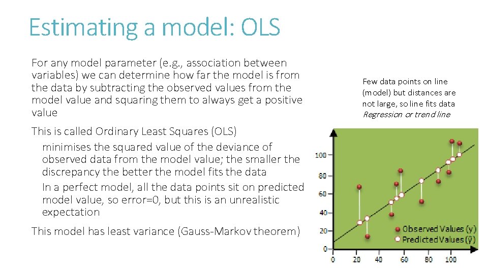
Estimating a model: OLS For any model parameter (e. g. , association between variables) we can determine how far the model is from the data by subtracting the observed values from the model value and squaring them to always get a positive value This is called Ordinary Least Squares (OLS) minimises the squared value of the deviance of observed data from the model value; the smaller the discrepancy the better the model fits the data In a perfect model, all the data points sit on predicted model value, so error=0, but this is an unrealistic expectation This model has least variance (Gauss-Markov theorem) Few data points on line (model) but distances are not large, so line fits data Regression or trend line

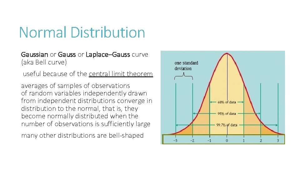
Normal Distribution Gaussian or Gauss or Laplace–Gauss curve (aka Bell curve) useful because of the central limit theorem averages of samples of observations of random variables independently drawn from independent distributions converge in distribution to the normal, that is, they become normally distributed when the number of observations is sufficiently large many other distributions are bell-shaped

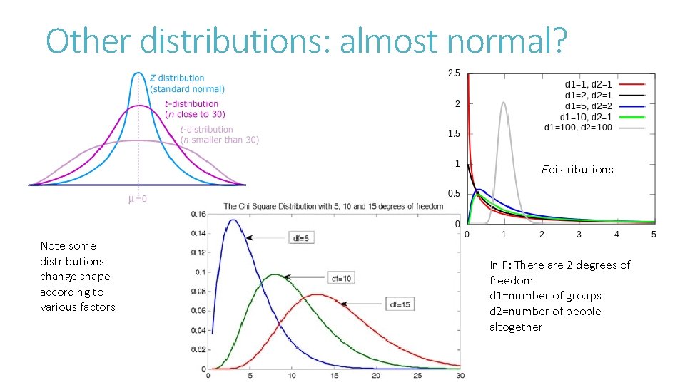
Other distributions: almost normal? F distributions Note some distributions change shape according to various factors In F: There are 2 degrees of freedom d 1=number of groups d 2=number of people altogether

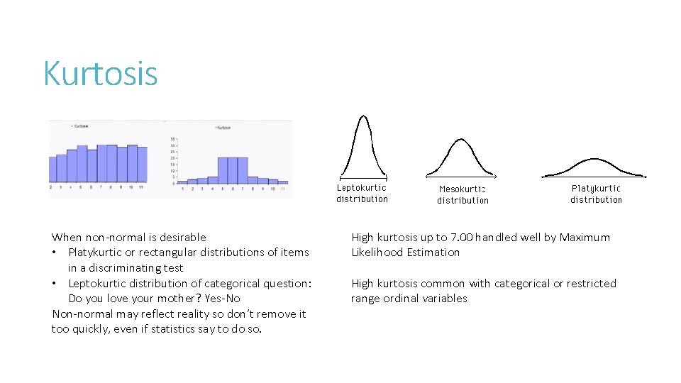
Kurtosis When non-normal is desirable • Platykurtic or rectangular distributions of items in a discriminating test • Leptokurtic distribution of categorical question: Do you love your mother? Yes-No Non-normal may reflect reality so don’t remove it too quickly, even if statistics say to do so. High kurtosis up to 7. 00 handled well by Maximum Likelihood Estimation High kurtosis common with categorical or restricted range ordinal variables

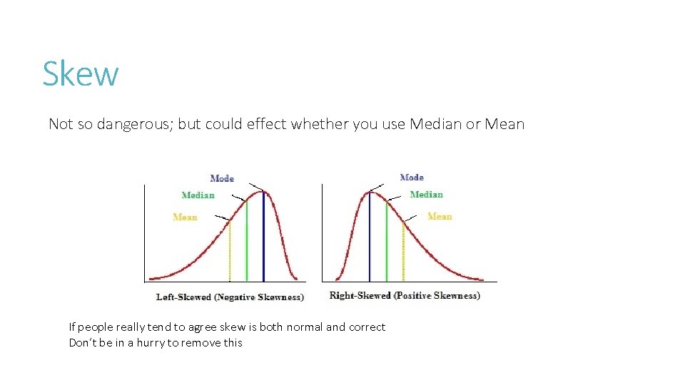
Skew Not so dangerous; but could effect whether you use Median or Mean If people really tend to agree skew is both normal and correct Don’t be in a hurry to remove this

Normality of Distributions With large enough sample sizes (>30 or 40), the violation of the normality assumption should not cause major problems; this implies that we can use parametric procedures even when the data are not normally distributed. With 100 s distributions don’t matter because of the central limit theorem, (a) if the sample data are approximately normal then the sampling distribution too will be normal; (b) in large samples (>30 or 40), the sampling distribution tends to be normal, regardless of the shape of the data; and (c) means of random samples from any distribution will themselves have normal distribution. Ghasemi, A. , & Zahediasl, S. (2012). Normality Tests for Statistical Analysis: A Guide for Non-Statisticians. International Journal of Endocrinology and Metabolism, 10(2), 486 -489. 10. 5812/ijem. 3505

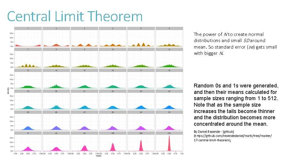
Central Limit Theorem The power of N to create normal distributions and small SD around mean. So standard error (se) gets small with bigger N. Random 0 s and 1 s were generated, and then their means calculated for sample sizes ranging from 1 to 512. Note that as the sample size increases the tails become thinner and the distribution becomes more concentrated around the mean. By Daniel Resende - [github] (https: //github. com/resendedaniel/math/tree/master/ 17 -central-limit-theorem),

What to do Therefore, critical values for rejecting the null hypothesis need to be different according to the sample size as follows: For small samples (n < 50), if absolute z-scores for either skewness or kurtosis are >1. 96, which corresponds with a alpha level 0. 05, then reject the null hypothesis and conclude the distribution of the sample is non-normal. For medium-sized samples (50 < n < 300), reject the null hypothesis at absolute zvalue >3. 29, which corresponds with a alpha level 0. 05, and conclude the distribution of the sample is non-normal. For sample sizes >300, depend on the histograms and the absolute values of skewness and kurtosis without considering z-values. Either an absolute skew value larger than 2 or an absolute kurtosis (proper) larger than 7 may be used as reference values for determining substantial non-normality. Kim, H. -Y. (2013). Statistical notes for clinical researchers: assessing normal distribution (2) using skewness and kurtosis. Restorative Dentistry & Endodontics, 38(1), 52– 54. http: //doi. org/10. 5395/rde. 2013. 38. 1. 52

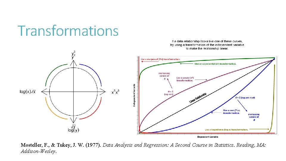
Transformations Mosteller, F. , & Tukey, J. W. (1977). Data Analysis and Regression: A Second Course in Statistics. Reading, MA: Addison-Wesley.

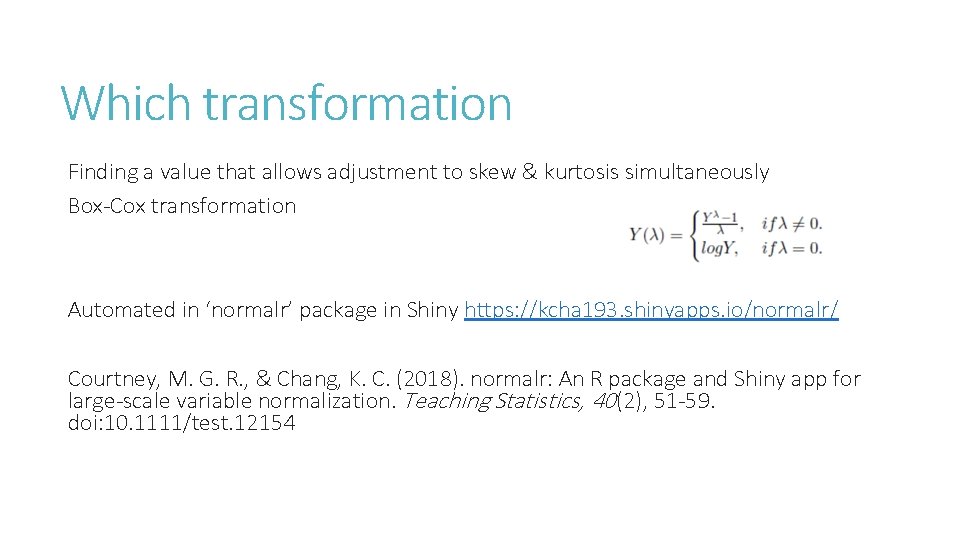
Which transformation Finding a value that allows adjustment to skew & kurtosis simultaneously Box-Cox transformation Automated in ‘normalr’ package in Shiny https: //kcha 193. shinyapps. io/normalr/ Courtney, M. G. R. , & Chang, K. C. (2018). normalr: An R package and Shiny app for large-scale variable normalization. Teaching Statistics, 40 (2), 51 -59. doi: 10. 1111/test. 12154

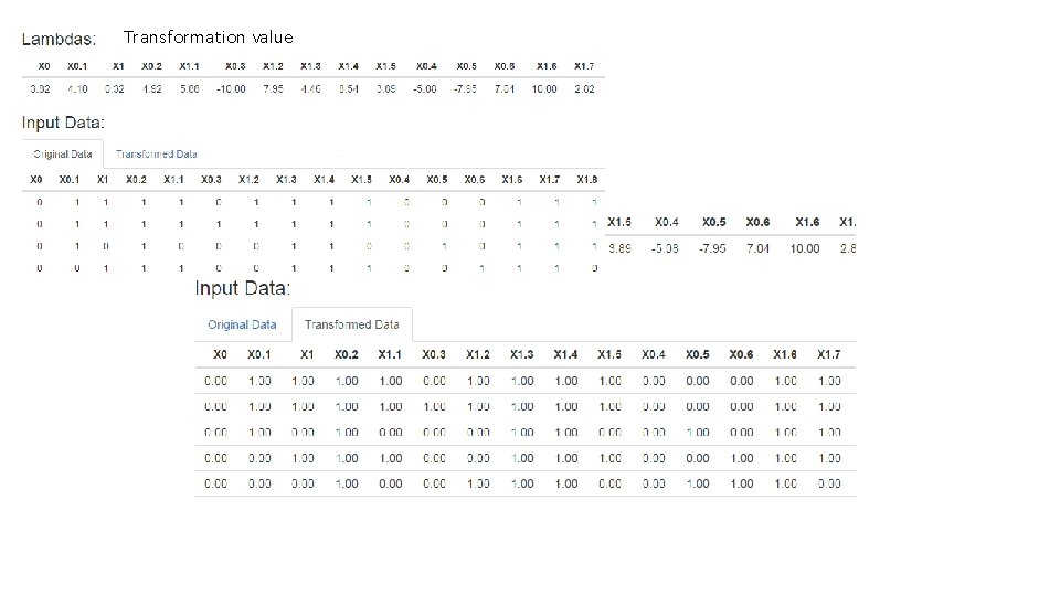
Transformation value

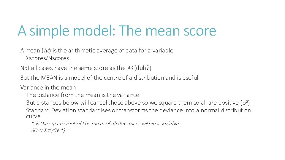
A simple model: The mean score A mean (M) is the arithmetic average of data for a variable Σscores/Nscores Not all cases have the same score as the M (duh? ) But the MEAN is a model of the centre of a distribution and is useful Variance in the mean The distance from the mean is the variance But distances below will cancel those above so we square them so all are positive (σ2) Standard Deviation standardises or transforms the deviance into a normal distribution curve It is the square root of the mean of all deviances within a variable SD=√ Σσ2/(N-1)

Point estimate The value we calculate from our samples is a point estimate There is actually a range in which highly plausible values would occur if our sampling had been different (standard error) Also to be reasonably sure of the true value, we should account for the error caused by sampling Now we can create an interval (range) which depicts how confident we are that the true value has been captured Remember margin of error?

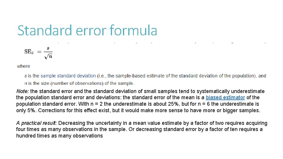
Standard error formula Note: the standard error and the standard deviation of small samples tend to systematically underestimate the population standard error and deviations: the standard error of the mean is a biased estimator of the population standard error. With n = 2 the underestimate is about 25%, but for n = 6 the underestimate is only 5%. Corrections for this effect exist, but it would make more sense to have more or bigger samples. A practical result: Decreasing the uncertainty in a mean value estimate by a factor of two requires acquiring four times as many observations in the sample. Or decreasing standard error by a factor of ten requires a hundred times as many observations

Confidence intervals An interval that communicates information regarding the probable magnitude of the point estimate μ When the sample mean is an estimator of the population mean, and the population is normally distributed, the sample mean will be normally distributed 95% confidence interval (95 CI) in a NORMAL distribution is the M +/- 2 SD; so we can be pretty sure (α=. 05) that the range includes the mean

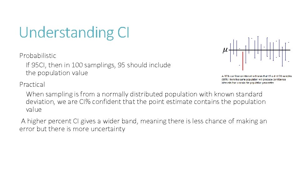
Understanding CI Probabilistic If 95 CI, then in 100 samplings, 95 should include the population value Practical When sampling is from a normally distributed population with known standard deviation, we are CI% confident that the point estimate contains the population value A higher percent CI gives a wider band, meaning there is less chance of making an error but there is more uncertainty

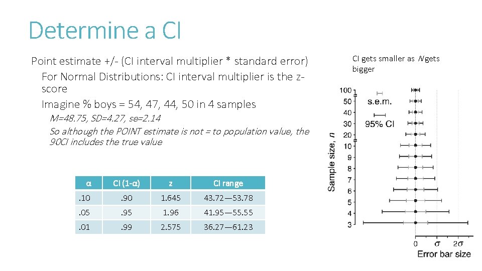
Determine a CI Point estimate +/- (CI interval multiplier * standard error) For Normal Distributions: CI interval multiplier is the zscore Imagine % boys = 54, 47, 44, 50 in 4 samples M=48. 75, SD=4. 27, se=2. 14 So although the POINT estimate is not = to population value, the 90 CI includes the true value α CI (1 -α) z CI range . 10 . 90 1. 645 43. 72— 53. 78 . 05 . 95 1. 96 41. 95— 55. 55 . 01 . 99 2. 575 36. 27— 61. 23 CI gets smaller as N gets bigger

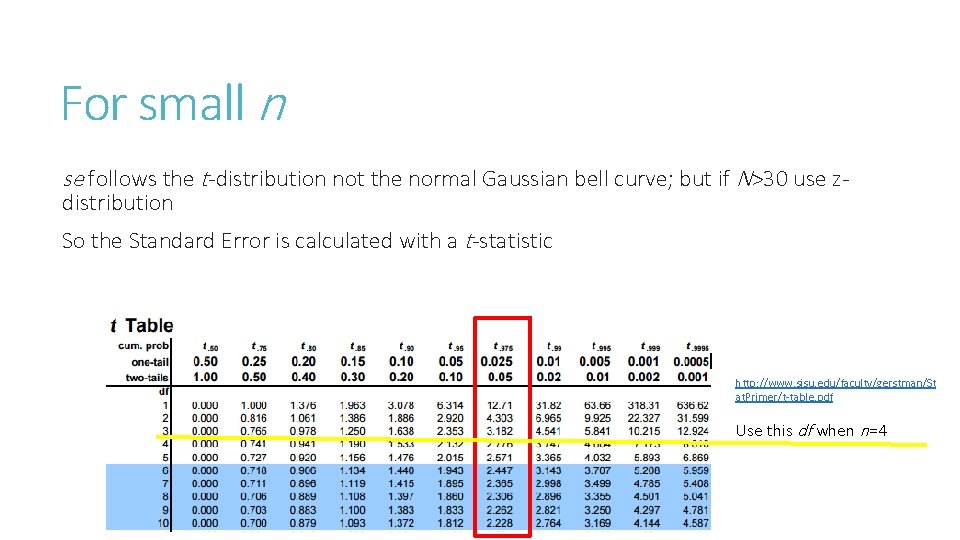
For small n se follows the t-distribution not the normal Gaussian bell curve; but if N>30 use zdistribution So the Standard Error is calculated with a t-statistic http: //www. sjsu. edu/faculty/gerstman/St at. Primer/t-table. pdf Use this df when n=4

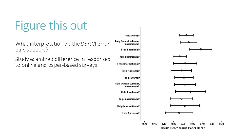
Figure this out What interpretation do the 95%CI error bars support? Study examined difference in responses to online and paper-based surveys.

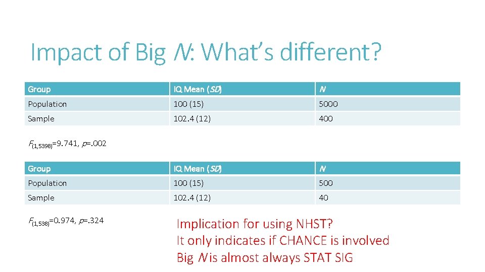
Impact of Big N: What’s different? Group IQ Mean (SD) N Population 100 (15) 5000 Sample 102. 4 (12) 400 Group IQ Mean (SD) N Population 100 (15) 500 Sample 102. 4 (12) 40 F(1, 5398)=9. 741, p=. 002 F(1, 538)=0. 974, p=. 324 Implication for using NHST? It only indicates if CHANCE is involved Big N is almost always STAT SIG

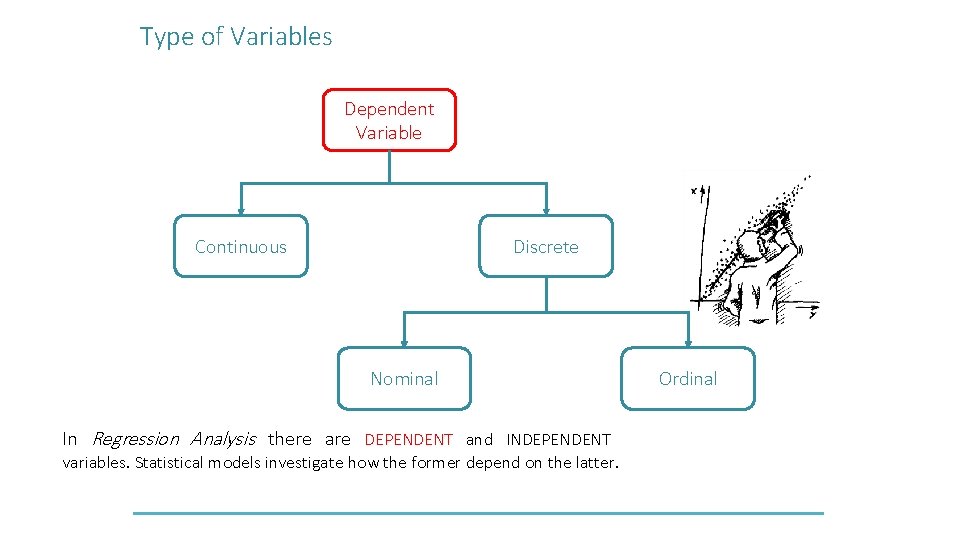
Type of Variables Dependent Variable Continuous Discrete Nominal In Regression Analysis there are DEPENDENT and INDEPENDENT variables. Statistical models investigate how the former depend on the latter. Ordinal

Prediction, Causation, Association Most common models assume linear (i. e. , correlations and regressions) relationships (paths) exist among constructs. a straight line relationship exists between variables and is sufficient basis for modeling how these things inter-relate Linearity requires a plausible causal mechanism…. Linear relations can be diagrammed and statistically calculated provided enough data exists –does it work? And then the quality of the model to the data can be estimated---it works but is it worth keeping? Does it explain much?

Covariance measure of the joint variability of two or more random variables This shows how aligned variables are magnitude of the covariance is not easy to interpret because it is not normalized and depending on the magnitudes of the variables. The normalized version of the covariance, the Pearson correlation coefficient, however, shows by its magnitude the strength of the linear relation.

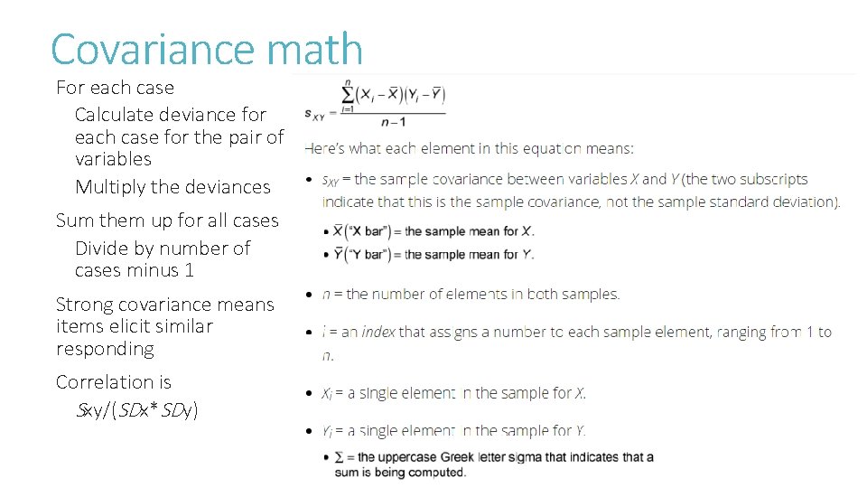
Covariance math For each case Calculate deviance for each case for the pair of variables Multiply the deviances Sum them up for all cases Divide by number of cases minus 1 Strong covariance means items elicit similar responding Correlation is Sxy/(SDx*SDy)

Correlations Synchronised patterns (A B) [2 or more things behave in a similar way] How big to be meaningful? How to qualitatively interpret values? When does a pattern really become visible? Weak: r<. 40 Moderate: . 40<r<. 70 Strong: r>. 70

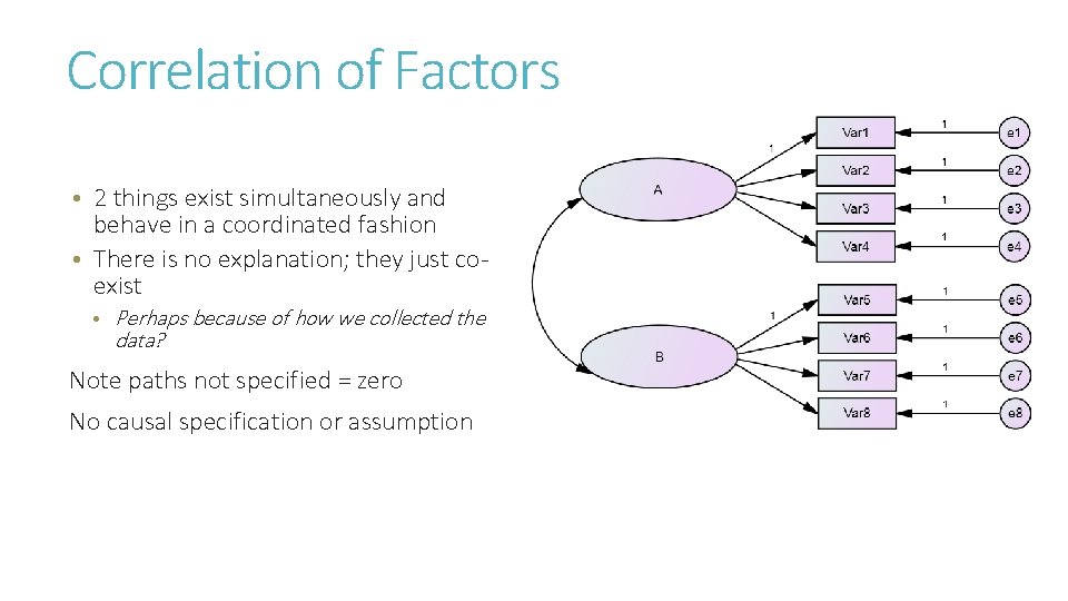
Correlation of Factors • 2 things exist simultaneously and behave in a coordinated fashion • There is no explanation; they just coexist • Perhaps because of how we collected the data? Note paths not specified = zero No causal specification or assumption

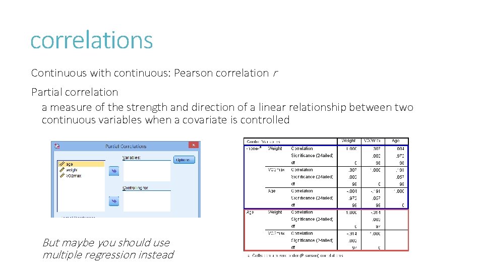
correlations Continuous with continuous: Pearson correlation r Partial correlation a measure of the strength and direction of a linear relationship between two continuous variables when a covariate is controlled But maybe you should use multiple regression instead

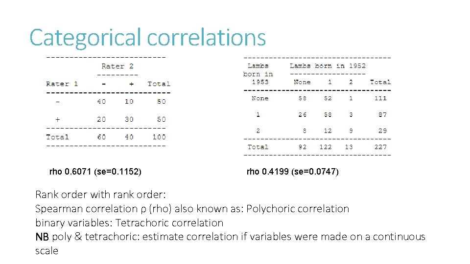
Categorical correlations rho 0. 6071 (se=0. 1152) rho 0. 4199 (se=0. 0747) Rank order with rank order: Spearman correlation ρ (rho) also known as: Polychoric correlation binary variables: Tetrachoric correlation NB poly & tetrachoric: estimate correlation if variables were made on a continuous scale

Why go further? Correlations are ultimately the raw material of fancier analyses so many reviewers or examiners want to see them But they don’t have much explanatory power—it’s just everything is connected and we don’t know which things matter Regression techniques at least allow one to create an argument that A causes B rather than simply describe that A is associated with B

Linearity: Regression b 1=slope [standardised beta = a proportion of standard deviation] b 0=intercept [starting point of equation; represents all the unknown stuff] Y variable Changes in X cause a linear change (increase or decrease) in YYY Formula: Y= m*X + b b 0 intercept e b 1: slop X variable Interpretations: 1. For every 1 SD change in X, you will get b 1*SDY change in Y. 2. This relationship explains m 2% of variance in Y

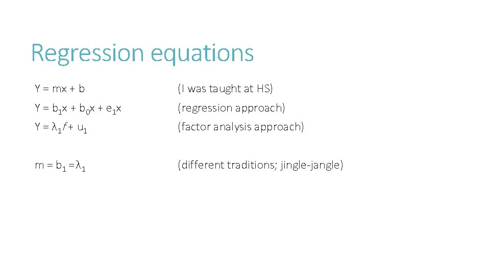
Regression equations Y = mx + b (I was taught at HS) Y = b 1 x + b 0 x + e 1 x (regression approach) Y = λ 1 f + u 1 (factor analysis approach) m = b 1 = λ 1 (different traditions; jingle-jangle)

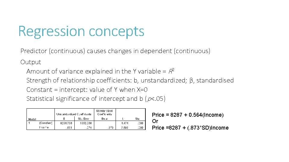
Regression concepts Predictor (continuous) causes changes in dependent (continuous) Output Amount of variance explained in the Y variable = R 2 Strength of relationship coefficients: b, unstandardized; β, standardised Constant = intercept: value of Y when X=0 Statistical significance of intercept and b (p<. 05) Price = 8287 + 0. 564(Income) Or Price =8287 + (. 873*SD)Income

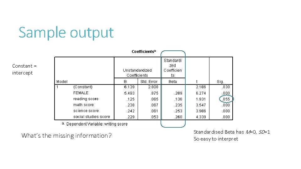
Sample output Constant = intercept What’s the missing information? Standardised Beta has M=0, SD=1 So easy to interpret

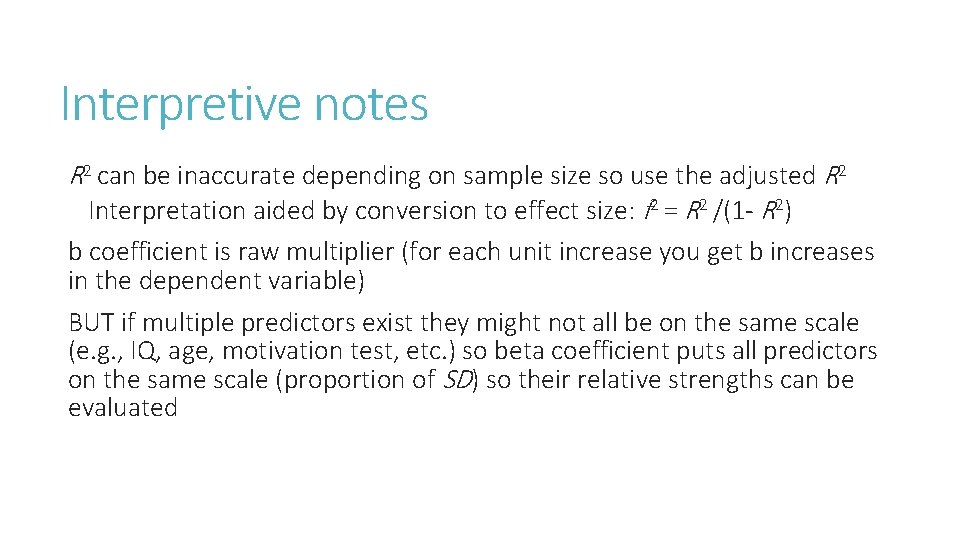
Interpretive notes R 2 can be inaccurate depending on sample size so use the adjusted R 2 Interpretation aided by conversion to effect size: f 2 = R 2 /(1 - R 2) b coefficient is raw multiplier (for each unit increase you get b increases in the dependent variable) BUT if multiple predictors exist they might not all be on the same scale (e. g. , IQ, age, motivation test, etc. ) so beta coefficient puts all predictors on the same scale (proportion of SD) so their relative strengths can be evaluated

Regression Multiple IV predict 1 DV Handles better possible overlap among IV (eliminates problem that every univariate variable is stat sig) Sequence of Adding predictors important Simultaneous (all at once; focused on individual unique contribution) Hierarchical (analyst specified order of introduction, sometimes in blocks; should belogically or theoretically grouped) Demographics; control variables; variables of interest Step-wise (data mining technique; machine identifies DV that predicts most to least and removes those not adding any value)

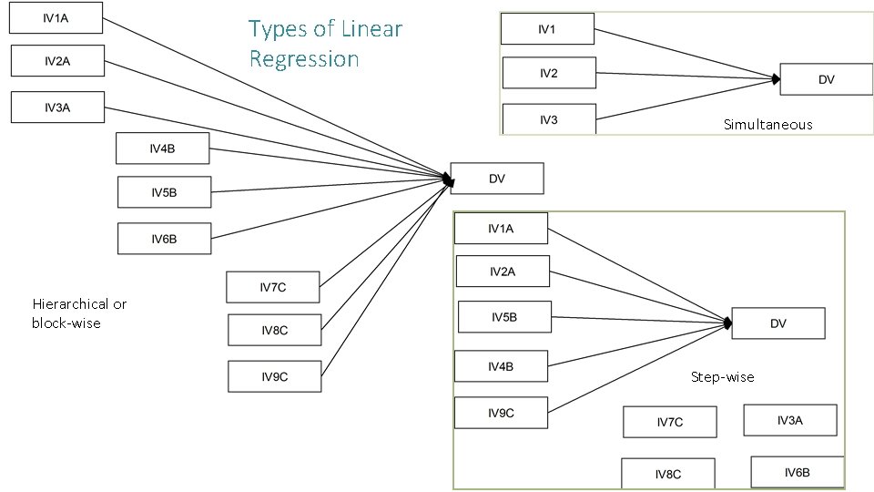
Types of Linear Regression Simultaneous Hierarchical or block-wise Step-wise

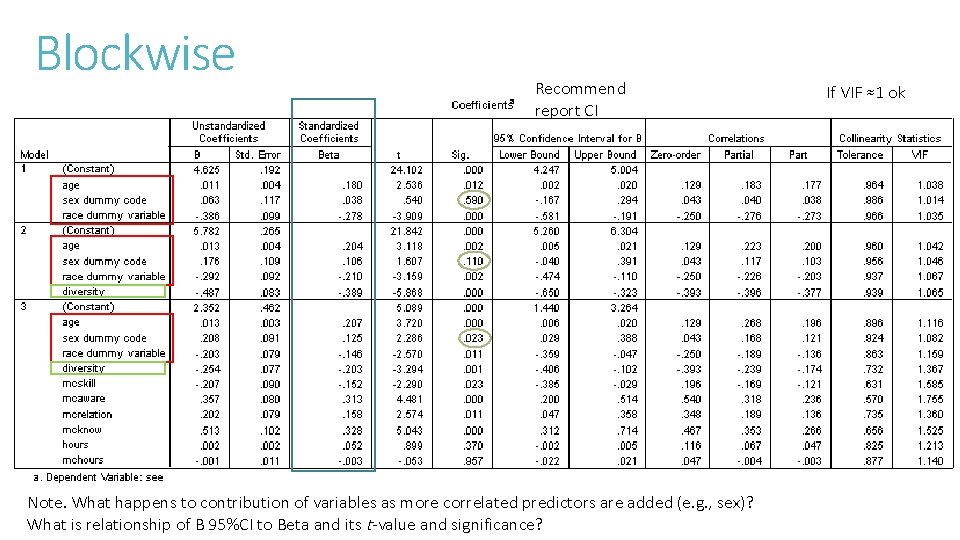
Blockwise Recommend report CI Note. What happens to contribution of variables as more correlated predictors are added (e. g. , sex)? What is relationship of B 95%CI to Beta and its t-value and significance? If VIF ≈1 ok

Impact of Predictors Proportion of variance explained by the predictors R 2 Square the standardised beta weight of the predictor to get R 2 If multiple predictors then the sum of squares will be R 2 the R 2 value is sometimes called the squared multiple correlation (SMC) If predictors are correlated then the sum of SMC may be smaller than actual individual contribution because of shared variance in the IV Remember STAT SIG is easy if N is big; what matters is explanatory power NB. The value of beta in a regression is identical to the value of r in a correlation Hierarchical: How much extra variance is achieved in DV by addition of additional predictors? If nothing more then additional predictors not needed.

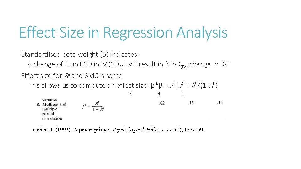
Effect Size in Regression Analysis Standardised beta weight (β) indicates: A change of 1 unit SD in IV (SDIV) will result in β*SD(IV) change in DV Effect size for R 2 and SMC is same This allows us to compute an effect size: β*β = R 2; f 2 = R 2/(1 -R 2) S M L Cohen, J. (1992). A power primer. Psychological Bulletin, 112(1), 155 -159.

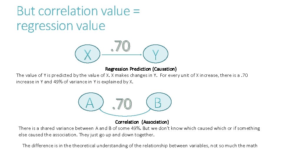
But correlation value = regression value . 70 Regression Prediction (Causation) The value of Y is predicted by the value of X. X makes changes in Y. For every unit of X increase, there is a. 70 increase in Y and 49% of variance in Y is explained by X. . 70 Correlation (Association) There is a shared variance between A and B of some 49%. But we don’t know which caused which or if something else caused the association. They just go up and down together. The difference is in theoretical understanding of the relationship between variables, not so much the math

Is it proof? The regression model is causal Increase in A causes change in B But is it proof? Unless you have a causal design and a causal mechanism it is NOT proof It is indicative, suggestive and possibly the basis for further research But mathematically & statistically it looks like causal proof Be prepared for critique

Disentangling association from causation Just because 2 things are related does not make one of them causal of the other Positive correlation between ice cream consumption and drowning murder boating accidents shark attacks But ice cream eating does not cause these events to take place HOWEVER, warm weather is associated with ice cream eating and the other events

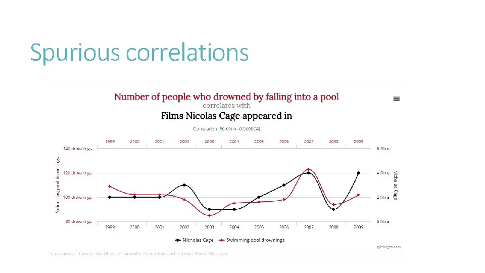
Spurious correlations

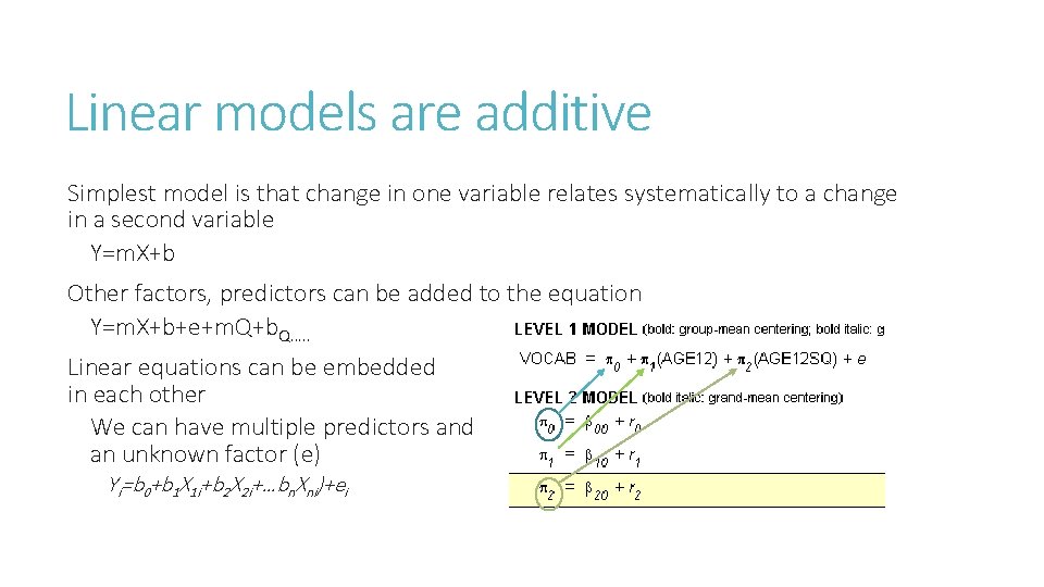
Linear models are additive Simplest model is that change in one variable relates systematically to a change in a second variable Y=m. X+b Other factors, predictors can be added to the equation Y=m. X+b+e+m. Q+b. Q…. . Linear equations can be embedded in each other We can have multiple predictors and an unknown factor (e) Yi=b 0+b 1 X 1 i+b 2 X 2 i+…bn. Xni)+ei

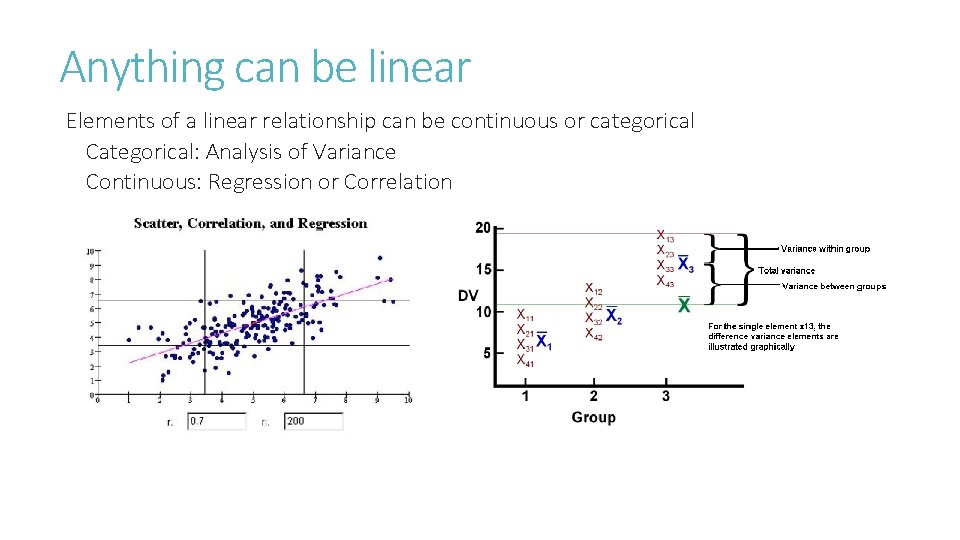
Anything can be linear Elements of a linear relationship can be continuous or categorical Categorical: Analysis of Variance Continuous: Regression or Correlation

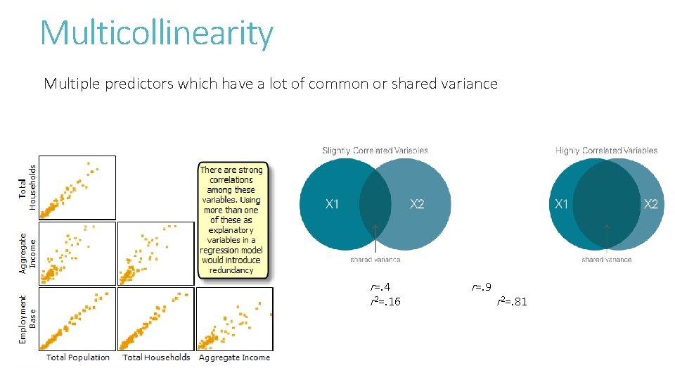
Multicollinearity Multiple predictors which have a lot of common or shared variance r=. 4 r 2=. 16 r=. 9 r 2=. 81

But even if multi-collinearity is not shown The tests and approaches of regular regression analysis might mask real relationships if you could control for residuals or the latent nature of variables HENCE Structural equation modeling

Differences in categorical distributions Do my participants have similar characteristics to the population? Did the splitting of groups into C and E create matched samples? Were the volunteers for next phase the same as those who didn’t volunteer? Basic test is the chi-square (χ2)

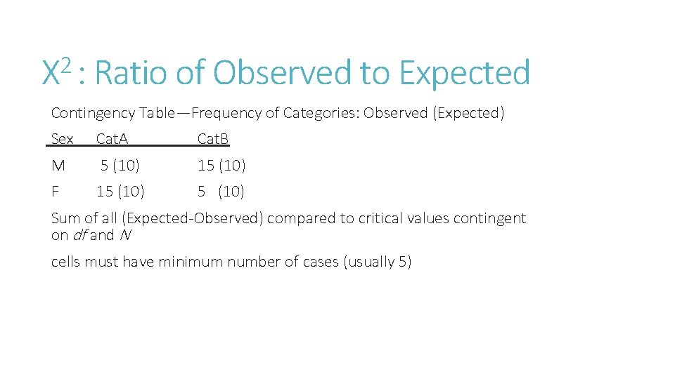
2 Χ : Ratio of Observed to Expected Contingency Table—Frequency of Categories: Observed (Expected) Sex Cat. A Cat. B M 5 (10) 15 (10) F 15 (10) Sum of all (Expected-Observed) compared to critical values contingent on df and N cells must have minimum number of cases (usually 5)

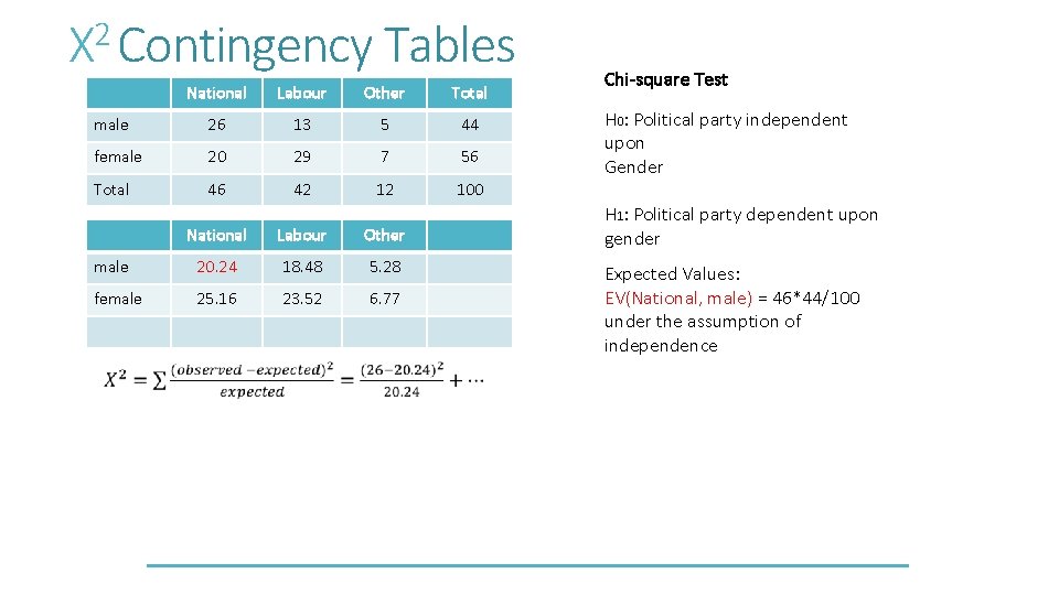
Χ 2 Contingency Tables National Labour Other Total male 26 13 5 44 female 20 29 7 56 Total 46 42 12 100 National Labour Other male 20. 24 18. 48 5. 28 female 25. 16 23. 52 6. 77 Chi-square Test H 0: Political party independent upon Gender H 1: Political party dependent upon gender Expected Values: EV(National, male) = 46*44/100 under the assumption of independence

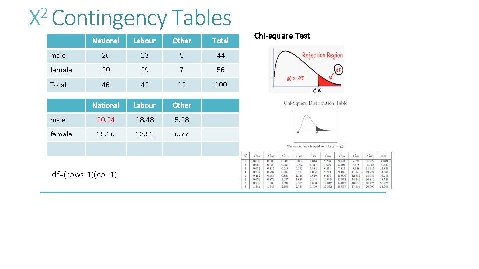
Χ 2 Contingency Tables National Labour Other Total male 26 13 5 44 female 20 29 7 56 Total 46 42 12 100 National Labour Other male 20. 24 18. 48 5. 28 female 25. 16 23. 52 6. 77 df=(rows-1)(col-1) Chi-square Test

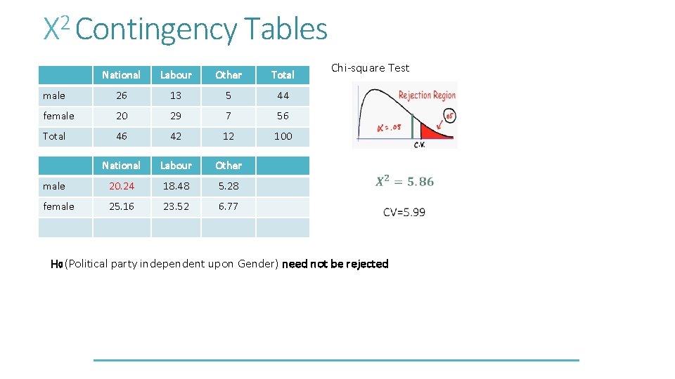
2 Χ Contingency Tables National Labour Other Total male 26 13 5 44 female 20 29 7 56 Total 46 42 12 100 National Labour Other male 20. 24 18. 48 5. 28 female 25. 16 23. 52 6. 77 Chi-square Test H 0 (Political party independent upon Gender) need not be rejected

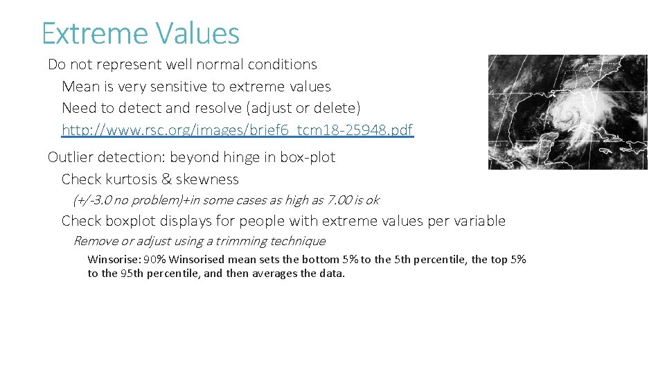
Extreme Values Do not represent well normal conditions Mean is very sensitive to extreme values Need to detect and resolve (adjust or delete) http: //www. rsc. org/images/brief 6_tcm 18 -25948. pdf Outlier detection: beyond hinge in box-plot Check kurtosis & skewness (+/-3. 0 no problem)+in some cases as high as 7. 00 is ok Check boxplot displays for people with extreme values per variable Remove or adjust using a trimming technique Winsorise: 90% Winsorised mean sets the bottom 5% to the 5 th percentile, the top 5% to the 95 th percentile, and then averages the data.

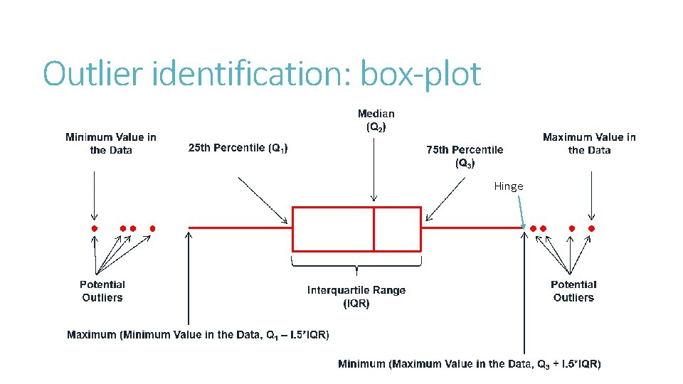
Outlier identification: box-plot Hinge

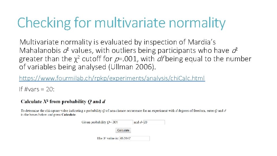
Checking for multivariate normality Multivariate normality is evaluated by inspection of Mardia’s Mahalanobis d 2 values, with outliers being participants who have d 2 greater than the χ2 cutoff for p=. 001, with df being equal to the number of variables being analysed (Ullman 2006). https: //www. fourmilab. ch/rpkp/experiments/analysis/chi. Calc. html If #vars = 20:

Outliers: When in doubt However, deletion of outlying participants, while permitting analysis within assumptions of the method, should not be automatic; because within large samples, legitimate extreme cases will be included in the sampling frame (Osborne and Overbay 2004). It makes sense to evaluate a model both with and without the outliers to determine whether deletion makes a difference to fit quality; a statistically significant difference in the Akaike information criterion (AIC) can be used to identify superior fit (Burnham and Anderson 2004). Test it both ways. Sensitivity analysis

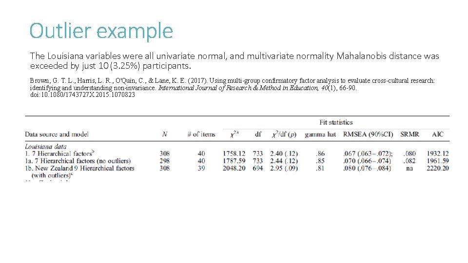
Outlier example The Louisiana variables were all univariate normal, and multivariate normality Mahalanobis distance was exceeded by just 10 (3. 25%) participants. Brown, G. T. L. , Harris, L. R. , O'Quin, C. , & Lane, K. E. (2017). Using multi-group confirmatory factor analysis to evaluate cross-cultural research: identifying and understanding non-invariance. International Journal of Research & Method in Education, 40(1), 66 -90. doi: 10. 1080/1743727 X. 2015. 1070823

Another sensitivity analysis a small, quasi-experimental, pre-post-test study of reading vocabulary (Sorrell, 2013). one student in an experimental group (n=7) of 2 nd grade students was an outlier, A paired-samples t-test with (t(6)=8. 78, p<. 001) and without (t(5)=7. 61, p=. 001) the outlier case was statistically significant for both conditions, though somewhat smaller without this case. effect size with the case (d=1. 53) was considerably larger than without the case (d=1. 00), although in both cases the effect was large. Removing the outlier provided a smaller estimate of effect, it is probably more defensible to accept this as the ‘truer’ estimate of the intervention effect. Sorrell, D. (2013). A study of achievement in English for students learning within a curriculum taught in their second language in a Hong Kong international school. (Ed. D Unpublished doctoral dissertation), Hong Kong Institute of Education, Hong Kong.