Review Intro Machine Learning Chapter 18 1 18

Review Intro Machine Learning Chapter 18. 1 -18. 4 • Understand Attributes, Target Variable, Error (loss) function, Classification & Regression, Hypothesis (Predictor) function • What is Supervised Learning? • Decision Tree Algorithm • Entropy & Information Gain • Tradeoff between train and test with model complexity • Cross validation

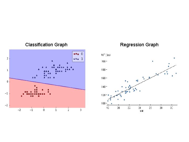
Supervised Learning • Use supervised learning – training data is given with correct output • We write program to reproduce this output with new test data • Eg : face detection • Classification : face detection, spam email • Regression : Netflix guesses how much you will rate the movie

Classification Graph Regression Graph

Terminology • Attributes – Also known as features, variables, independent variables, covariates • Target Variable – Also known as goal predicate, dependent variable, … • Classification – Also known as discrimination, supervised classification, … • Error function – Also known as objective function, loss function, …

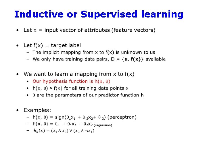
Inductive or Supervised learning

Empirical Error Functions • E(h) = x distance[h(x, ) , f(x)] Sum is over all training pairs in the training data D Examples: distance = squared error if h and f are real-valued (regression) distance = delta-function if h and f are categorical (classification) In learning, we get to choose 1. what class of functions h(. . ) we want to learn – potentially a huge space! (“hypothesis space”) 2. what error function/distance we want to use - should be chosen to reflect real “loss” in problem - but often chosen for mathematical/algorithmic convenience

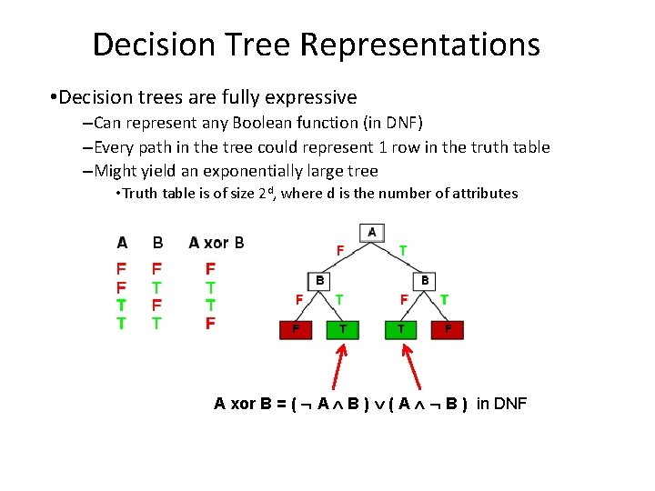
Decision Tree Representations • Decision trees are fully expressive –Can represent any Boolean function (in DNF) –Every path in the tree could represent 1 row in the truth table –Might yield an exponentially large tree • Truth table is of size 2 d, where d is the number of attributes A xor B = ( A B ) ( A B ) in DNF

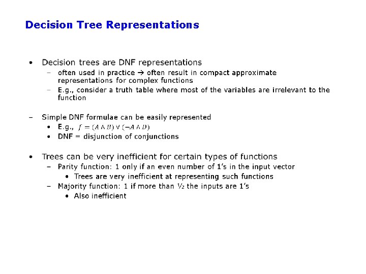
Decision Tree Representations

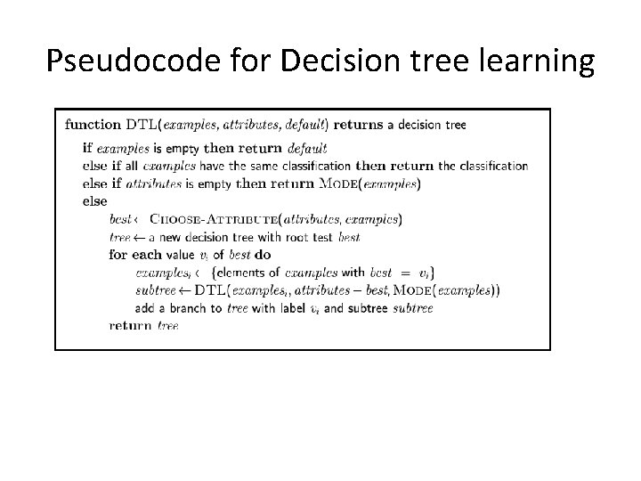
Pseudocode for Decision tree learning

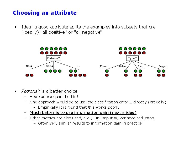
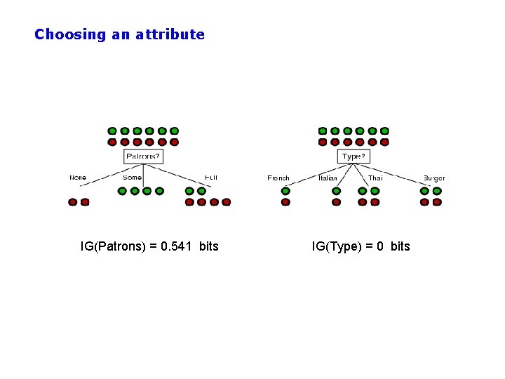
Choosing an attribute • Idea: a good attribute splits the examples into subsets that are (ideally) "all positive" or "all negative" • Patrons? is a better choice – How can we quantify this? – One approach would be to use the classification error E directly (greedily) • Empirically it is found that this works poorly – Much better is to use information gain (next slides) – Other metrics are also used, e. g. , Gini impurity, variance reduction – Often very similar results to information gain in practice

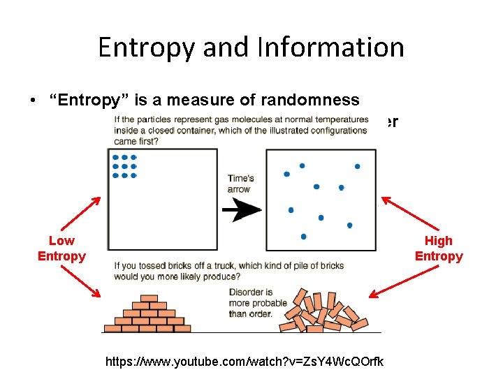
Entropy and Information • “Entropy” is a measure of randomness = amount of disorder High Entropy Low Entropy https: //www. youtube. com/watch? v=Zs. Y 4 Wc. QOrfk

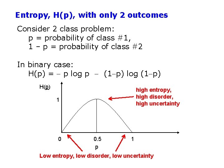
Entropy, H(p), with only 2 outcomes Consider 2 class problem: p = probability of class #1, 1 – p = probability of class #2 In binary case: H(p) = p log p (1 p) log (1 p) H(p) high entropy, high disorder, high uncertainty 1 0 0. 5 p 1 Low entropy, low disorder, low uncertainty

Entropy and Information • Entropy H(X) = E[ log 1/P(X) ] = å x X P(x) log 1/P(x) = −å x X P(x) log P(x) – Log base two, units of entropy are “bits” – If only two outcomes: H(p) = p log(p) (1 p) log(1 p) • Examples: H(x) =. 25 log 4 +. 25 log 4 = 2 bits Max entropy for 4 outcomes H(x) =. 75 log 4/3 +. 25 log 4 = 0. 8133 bits H(x) = 1 log 1 = 0 bits Min entropy

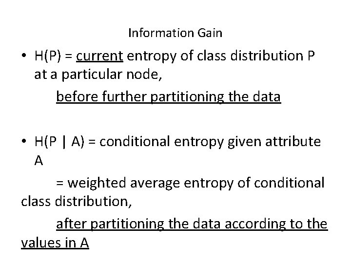
Information Gain • H(P) = current entropy of class distribution P at a particular node, before further partitioning the data • H(P | A) = conditional entropy given attribute A = weighted average entropy of conditional class distribution, after partitioning the data according to the values in A

Choosing an attribute IG(Patrons) = 0. 541 bits IG(Type) = 0 bits

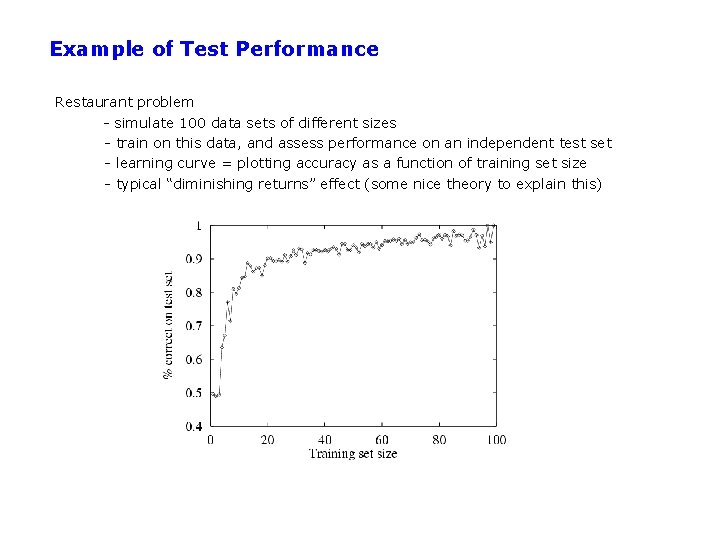
Example of Test Performance Restaurant problem - simulate 100 data sets of different sizes - train on this data, and assess performance on an independent test set - learning curve = plotting accuracy as a function of training set size - typical “diminishing returns” effect (some nice theory to explain this)

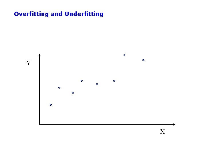
Overfitting and Underfitting Y X

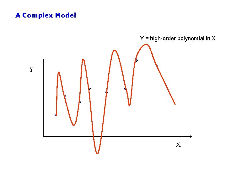
A Complex Model Y = high-order polynomial in X Y X

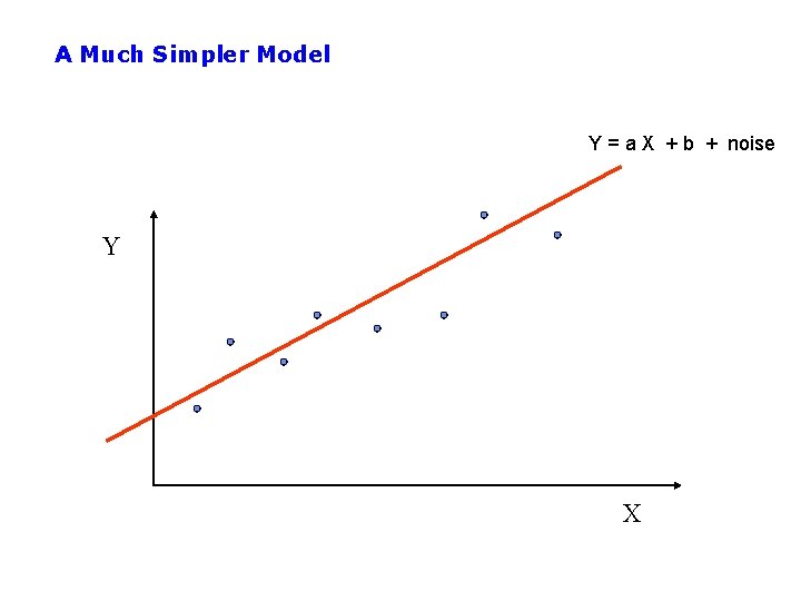
A Much Simpler Model Y = a X + b + noise Y X

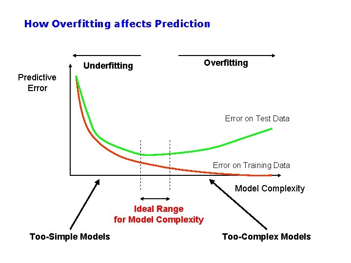
How Overfitting affects Prediction Underfitting Overfitting Predictive Error on Test Data Error on Training Data Model Complexity Ideal Range for Model Complexity Too-Simple Models Too-Complex Models

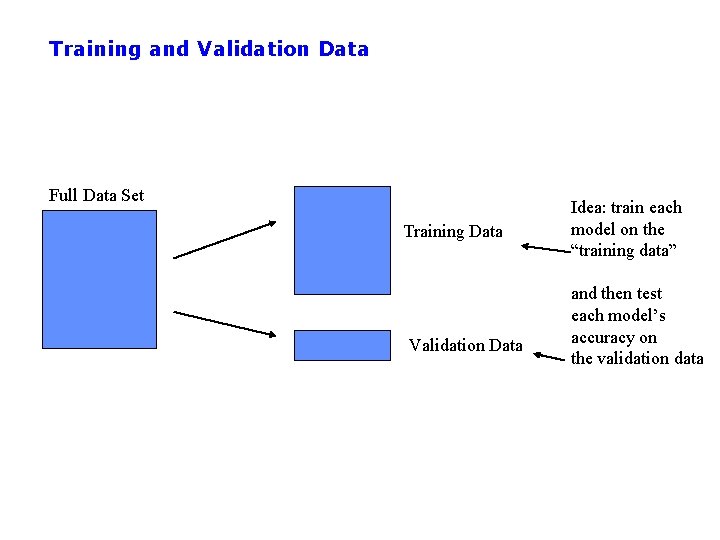
Training and Validation Data Full Data Set Training Data Validation Data Idea: train each model on the “training data” and then test each model’s accuracy on the validation data

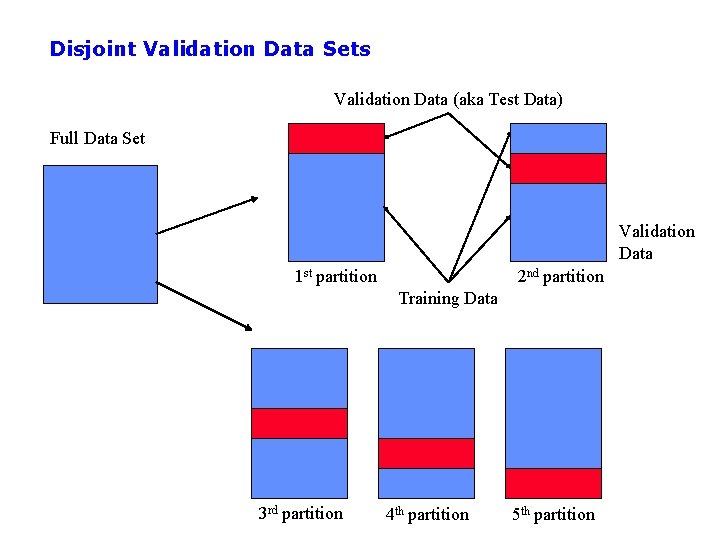
Disjoint Validation Data Sets Validation Data (aka Test Data) Full Data Set Validation Data 1 st partition 2 nd partition Training Data 3 rd partition 4 th partition 5 th partition

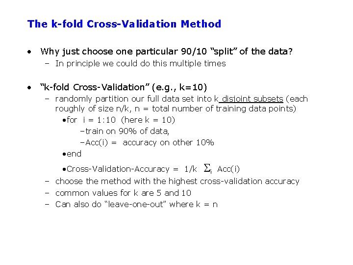
The k-fold Cross-Validation Method • Why just choose one particular 90/10 “split” of the data? – In principle we could do this multiple times • “k-fold Cross-Validation” (e. g. , k=10) – randomly partition our full data set into k disjoint subsets (each roughly of size n/k, n = total number of training data points) • for i = 1: 10 (here k = 10) –train on 90% of data, –Acc(i) = accuracy on other 10% • end • Cross-Validation-Accuracy = 1/k i Acc(i) – choose the method with the highest cross-validation accuracy – common values for k are 5 and 10 – Can also do “leave-one-out” where k = n

You will be expected to know Understand Attributes, Error function, Classification, Regression, Hypothesis (Predictor function) What is Supervised Learning? Decision Tree Algorithm Entropy Information Gain Tradeoff between train and test with model complexity Cross validation