Review for Final in ISQS 3344 Final will

Review for Final in ISQS 3344 Final will take place: Friday, July 8, 2016, 8: 00 am until 10: 30 am

Format b 100 -150 multiple choice worth 100% • 30 -50 of these are from previous segments of the course bexam is closed notes/closed book b. Exam will be comprehensive

Bring b Pencils b Calculator b Orange Scantron sheet

This exam will emphasize: b What we have covered since the second exam: • • Forecasting, Chapter 12 Sales and Operations Planning, Chapter 14 JIT and Lean Production, Chapter 16 Project Management, Chapter 9

OVERALL Content b We have covered Chapters 1, 2, 3, 4, 5, 6, 9, 10, 11 s, 12, 13 s, 14 s, 15 (ERP), and 16 b 3/4 ths of the test material will come from the last third of the course—Chapters 9, 12, 13, 14, 16 b Since a major theme of the course has been processes, review chapter 6 thoroughly

Problems in Multiple Choice b A FORECASTING PROBLEM LIKE 12 -10 b An aggregate planning (S&OP) PROBLEM LIKE 14 -6 b AN INVENTORY PROBLEM LIKE 13 -6 b Construct an activity on node network chart from a table; Determine duration, ES, EF, LS, LF and mark the critical path

FORECASTING--Two basic categories of approaches What are they? ?

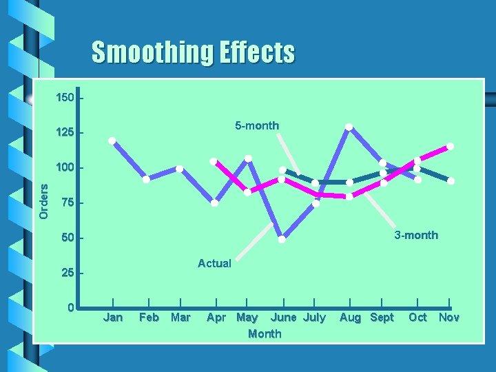
Smoothing Effects 150 – 5 -month 125 – Orders 100 – 75 – 3 -month 50 – Actual 25 – 0– | Jan | Feb | Mar | | Apr May June July Month | | Aug Sept | Oct | Nov

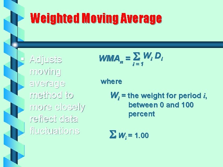
Weighted Moving Average § Adjusts moving average method to more closely reflect data fluctuations WMAn = Wi Di i=1 where Wi = the weight for period i, between 0 and 100 percent Wi = 1. 00

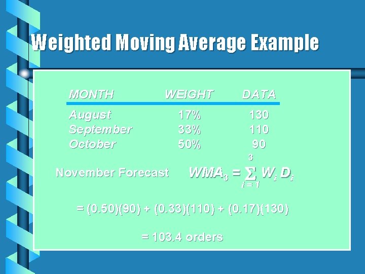
Weighted Moving Average Example MONTH WEIGHT DATA 17% 33% 50% 130 110 90 August September October 3 November Forecast WMA 3 = Wi Di i=1 = (0. 50)(90) + (0. 33)(110) + (0. 17)(130) = 103. 4 orders

Exponential Smoothing § § Averaging method Weights most recent data more strongly Reacts more to recent changes Widely used, accurate method

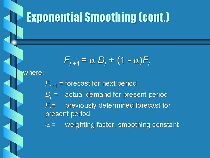
Exponential Smoothing (cont. ) Ft +1 = Dt + (1 - )Ft where: Ft +1 = forecast for next period Dt = actual demand for present period Ft = previously determined forecast for present period = weighting factor, smoothing constant

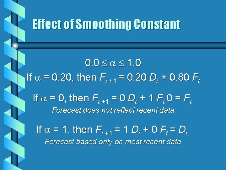
Effect of Smoothing Constant 0. 0 1. 0 If = 0. 20, then Ft +1 = 0. 20 Dt + 0. 80 Ft If = 0, then Ft +1 = 0 Dt + 1 Ft 0 = Ft Forecast does not reflect recent data If = 1, then Ft +1 = 1 Dt + 0 Ft = Dt Forecast based only on most recent data

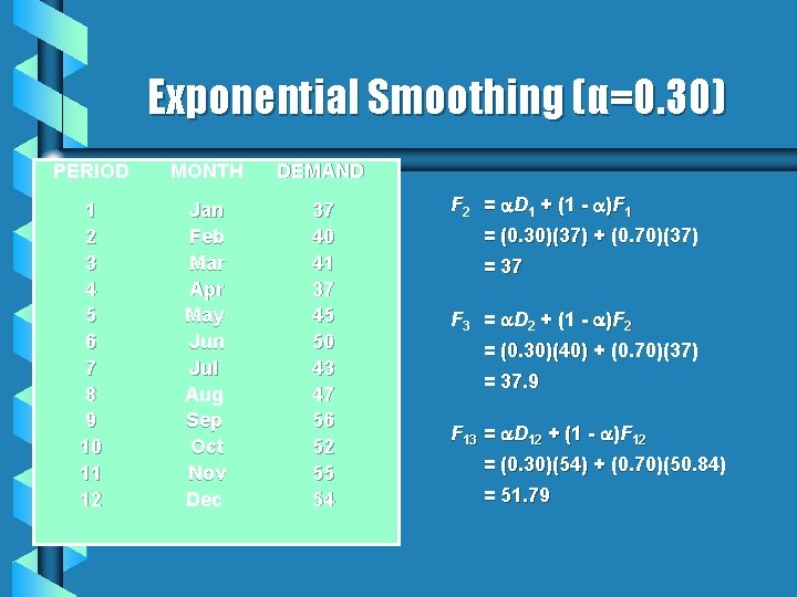
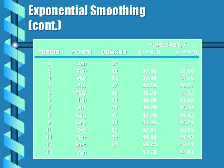
Exponential Smoothing (α=0. 30) PERIOD MONTH DEMAND 1 2 3 4 5 6 7 8 9 10 11 12 Jan Feb Mar Apr May Jun Jul Aug Sep Oct Nov Dec 37 40 41 37 45 50 43 47 56 52 55 54 F 2 = D 1 + (1 - )F 1 = (0. 30)(37) + (0. 70)(37) = 37 F 3 = D 2 + (1 - )F 2 = (0. 30)(40) + (0. 70)(37) = 37. 9 F 13 = D 12 + (1 - )F 12 = (0. 30)(54) + (0. 70)(50. 84) = 51. 79

Exponential Smoothing (cont. ) PERIOD MONTH DEMAND 1 2 3 4 5 6 7 8 9 10 11 12 13 Jan Feb Mar Apr May Jun Jul Aug Sep Oct Nov Dec Jan 37 40 41 37 45 50 43 47 56 52 55 54 – FORECAST, Ft + 1 ( = 0. 3) ( = 0. 5) – 37. 00 37. 90 38. 83 38. 28 40. 29 43. 20 43. 14 44. 30 47. 81 49. 06 50. 84 51. 79 – 37. 00 38. 50 39. 75 38. 37 41. 68 45. 84 44. 42 45. 71 50. 85 51. 42 53. 21 53. 61

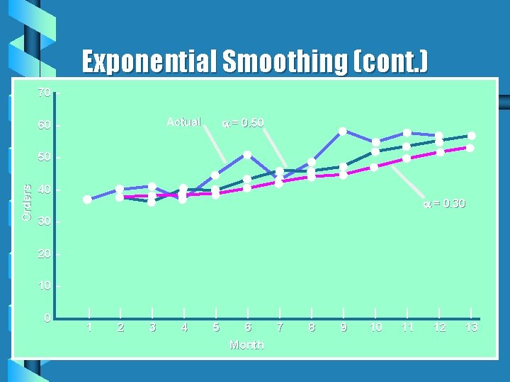
Exponential Smoothing (cont. ) 70 – = 0. 50 Actual 60 – Orders 50 – 40 – = 0. 30 30 – 20 – 10 – 0– | 1 | 2 | 3 | 4 | 5 | 6 Month | 7 | 8 | 9 | 10 | 11 | 12 | 13

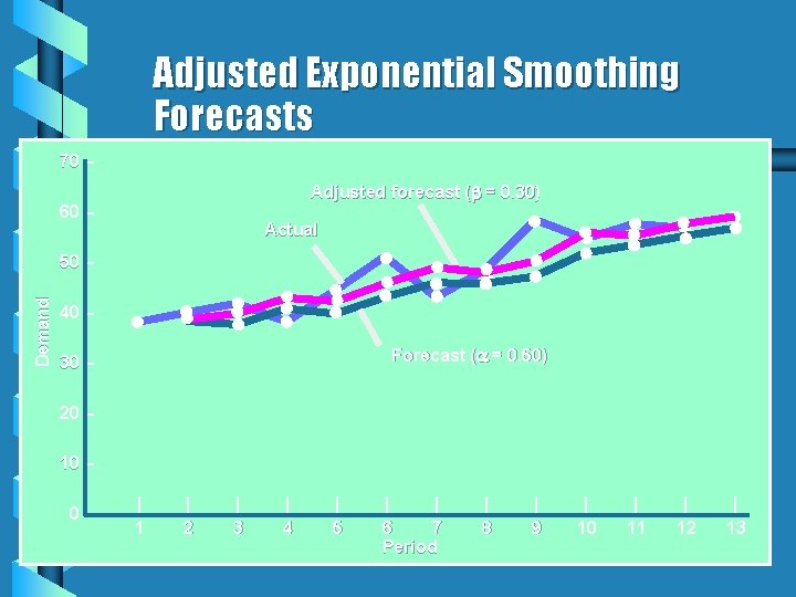
Adjusted Exponential Smoothing Forecasts 70 – Adjusted forecast ( = 0. 30) 60 – Actual Demand 50 – 40 – Forecast ( = 0. 50) 30 – 20 – 10 – 0– | 1 | 2 | 3 | 4 | 5 | | 6 7 Period | 8 | 9 | 10 | 11 | 12 | 13

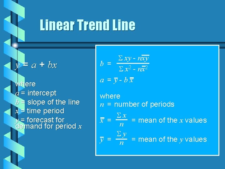
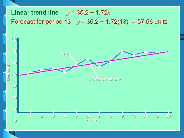
Linear Trend Line y = a + bx where a = intercept b = slope of the line x = time period y = forecast for demand for period x xy - nxy b = x 2 - nx 2 a = y-bx where n = number of periods x x = n = mean of the x values y y = n = mean of the y values

Linear trend line y = 35. 2 + 1. 72 x Forecast for period 13 y = 35. 2 + 1. 72(13) = 57. 56 units 70 – Demand 60 – Actual 50 – 40 – Linear trend line 30 – 20 – 10 – 0– | 1 | 2 | 3 | 4 | 5 | | 6 7 Period | 8 | 9 | 10 | 11 | 12 | 13

Advantages of Linear Trend Line b Very easy to do calculations in MS Excel b There is never any bias—consistently below or above the trend b Can forecast any number of periods out into the future • Cannot do this with weighted moving averages or with exponential smoothing

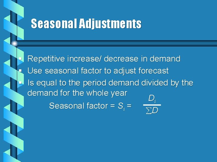
Seasonal Adjustments § Repetitive increase/ decrease in demand § Use seasonal factor to adjust forecast § Is equal to the period demand divided by the demand for the whole year Di Seasonal factor = Si = D

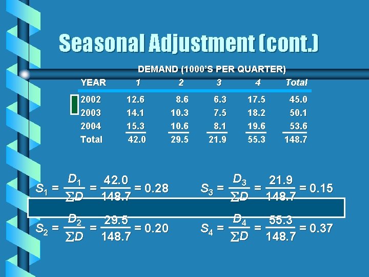
Seasonal Adjustment (cont. ) YEAR 2002 2003 2004 Total DEMAND (1000’S PER QUARTER) 1 2 3 4 Total 12. 6 14. 1 15. 3 42. 0 8. 6 10. 3 10. 6 29. 5 6. 3 7. 5 8. 1 21. 9 17. 5 18. 2 19. 6 55. 3 45. 0 50. 1 53. 6 148. 7 D 1 42. 0 S 1 = = = 0. 28 D 148. 7 D 3 21. 9 S 3 = = = 0. 15 D 148. 7 D 2 29. 5 S 2 = = = 0. 20 D 148. 7 D 4 55. 3 S 4 = = = 0. 37 D 148. 7

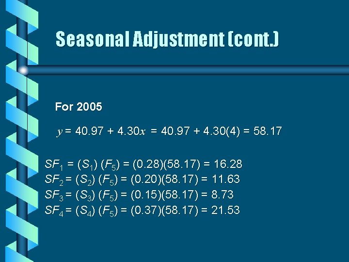
Seasonal Adjustment (cont. ) For 2005 y = 40. 97 + 4. 30 x = 40. 97 + 4. 30(4) = 58. 17 SF 1 = (S 1) (F 5) = (0. 28)(58. 17) = 16. 28 SF 2 = (S 2) (F 5) = (0. 20)(58. 17) = 11. 63 SF 3 = (S 3) (F 5) = (0. 15)(58. 17) = 8. 73 SF 4 = (S 4) (F 5) = (0. 37)(58. 17) = 21. 53

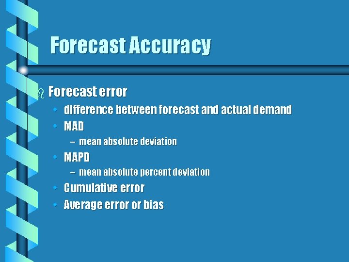
Forecast Accuracy b Forecast error • difference between forecast and actual demand • MAD – mean absolute deviation • MAPD – mean absolute percent deviation • Cumulative error • Average error or bias

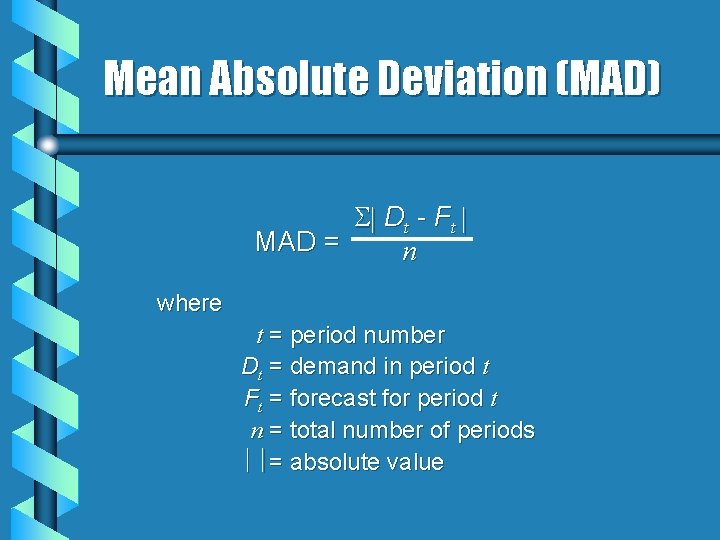
Mean Absolute Deviation (MAD) Dt - F t MAD = n where t = period number Dt = demand in period t Ft = forecast for period t n = total number of periods = absolute value

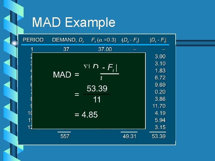
MAD Example

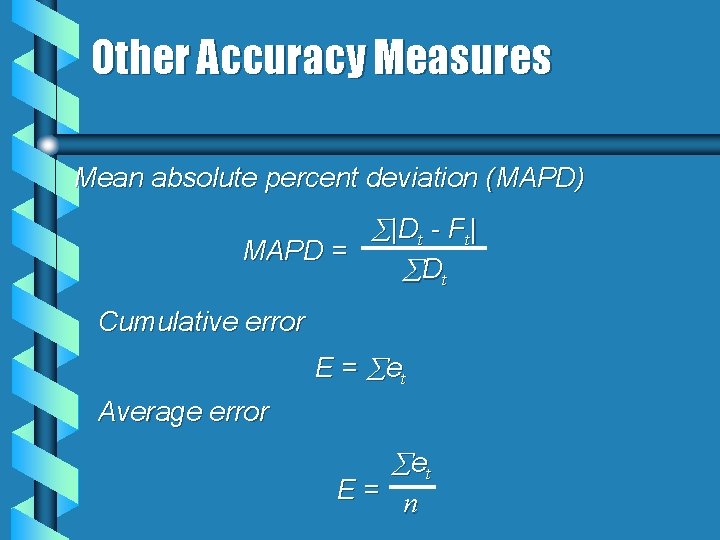
Other Accuracy Measures Mean absolute percent deviation (MAPD) |Dt - Ft| MAPD = Dt Cumulative error E = et Average error et E= n

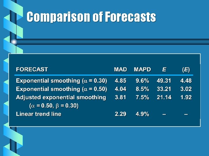
Comparison of Forecasts

Inventory Costs b Carrying or holding costs b Ordering costs b Stockout (shortage) costs b Back-ordering costs

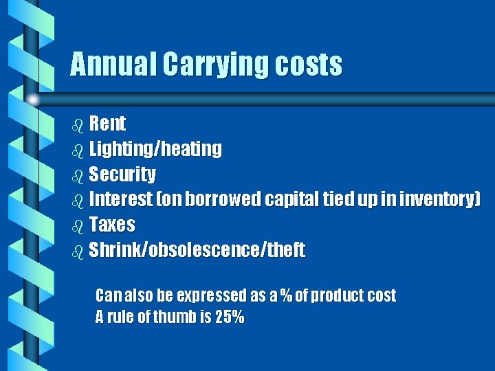
Annual Carrying costs b Rent b Lighting/heating b Security b Interest (on borrowed capital tied up in inventory) b Taxes b Shrink/obsolescence/theft Can also be expressed as a % of product cost A rule of thumb is 25%

Ordering costs—costs related to Transportation Costs Shipping Costs Receiving Costs Inspection Costs

Shortage costs b This is an opportunity cost b Is ignored in the simple inventory models, by assuming that there are no shortages b Consideration is given to shortages when we add safety stock to a Reorder Point, R = d*L + safety stock

What about shortage (out of stock) costs? ? b In the simple models we are looking at , we assume no shortages, no out of stock situations

Back-order costs? ? b We have back-order costs when we are out of stock and the customer is patient b Will assume impatient customers who must have the product they wish to buy NOW. b So back-ordering is not considered in the simple models we looked at

Chapter 14 –S&OP b S&OP – Sales and Operations Planning b Assumes an intermediate planning horizon — 6 to 24 months b S&OP gets marketing and operations (manufacturing) aligned and coordinated

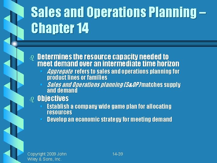
Sales and Operations Planning – Chapter 14 b Determines the resource capacity needed to meet demand over an intermediate time horizon • Aggregate refers to sales and operations planning for product lines or families • Sales and Operations planning (S&OP) matches supply and demand b Objectives • Establish a company wide game plan for allocating resources • Develop an economic strategy for meeting demand Copyright 2009 John Wiley & Sons, Inc. 14 -39

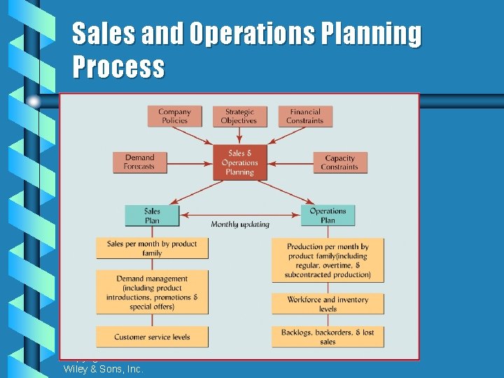
Sales and Operations Planning Process Copyright 2009 John Wiley & Sons, Inc. 14 -40

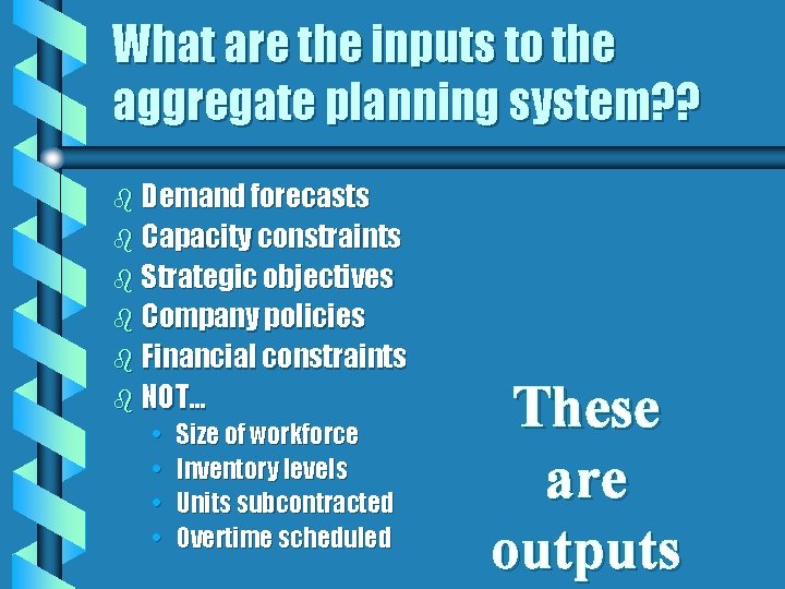
What are the inputs to the aggregate planning system? ? b Demand forecasts b Capacity constraints b Strategic objectives b Company policies b Financial constraints b NOT… • • Size of workforce Inventory levels Units subcontracted Overtime scheduled These are outputs

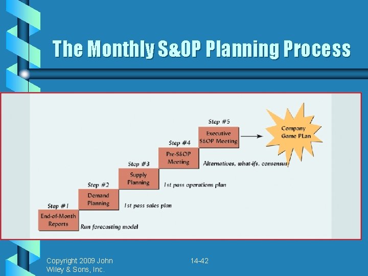
The Monthly S&OP Planning Process Copyright 2009 John Wiley & Sons, Inc. 14 -42

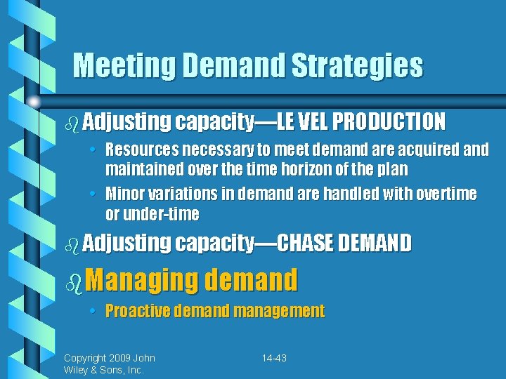
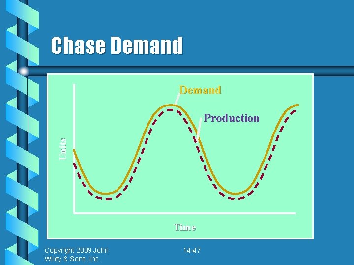
Meeting Demand Strategies b Adjusting capacity—LE VEL PRODUCTION • Resources necessary to meet demand are acquired and maintained over the time horizon of the plan • Minor variations in demand are handled with overtime or under-time b Adjusting capacity—CHASE DEMAND b. Managing demand • Proactive demand management Copyright 2009 John Wiley & Sons, Inc. 14 -43

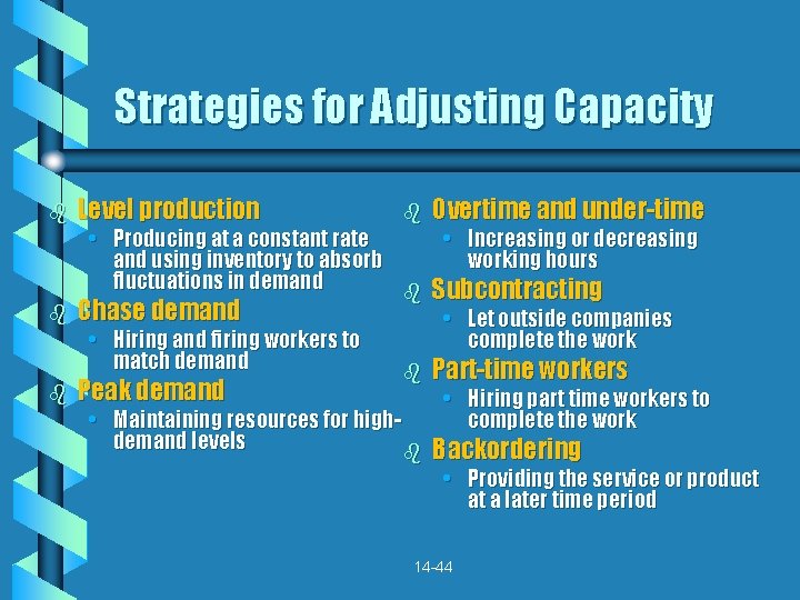
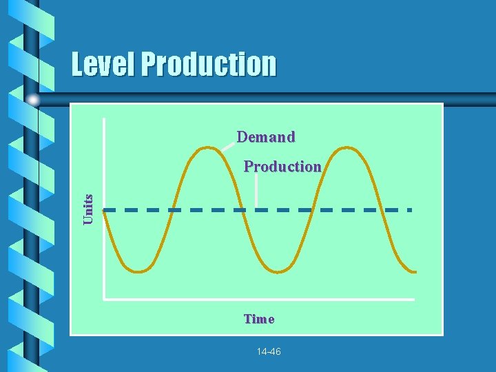
Strategies for Adjusting Capacity b Level production b Peak demand b Overtime and under-time • Producing at a constant rate • Increasing or decreasing and using inventory to absorb working hours fluctuations in demand b Subcontracting b Chase demand • Let outside companies • Hiring and firing workers to complete the work match demand b Part-time workers • Hiring part time workers to complete the work • Maintaining resources for highdemand levels b Backordering • Providing the service or product at a later time period 14 -44

Level Production Demand Units Production Time 14 -46

Chase Demand Units Production Time Copyright 2009 John Wiley & Sons, Inc. 14 -47

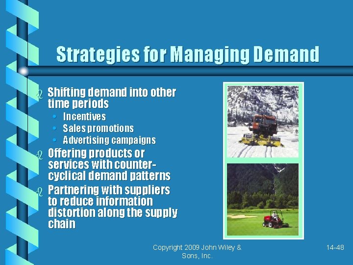
Strategies for Managing Demand b Shifting demand into other time periods • Incentives • Sales promotions • Advertising campaigns b b Offering products or services with countercyclical demand patterns Partnering with suppliers to reduce information distortion along the supply chain Copyright 2009 John Wiley & Sons, Inc. 14 -48

Quantitative Techniques For AP b Pure Strategies b Mixed Strategies b Linear Programming b Transportation Method b Other Quantitative Techniques Copyright 2009 John Wiley & Sons, Inc. 14 -49

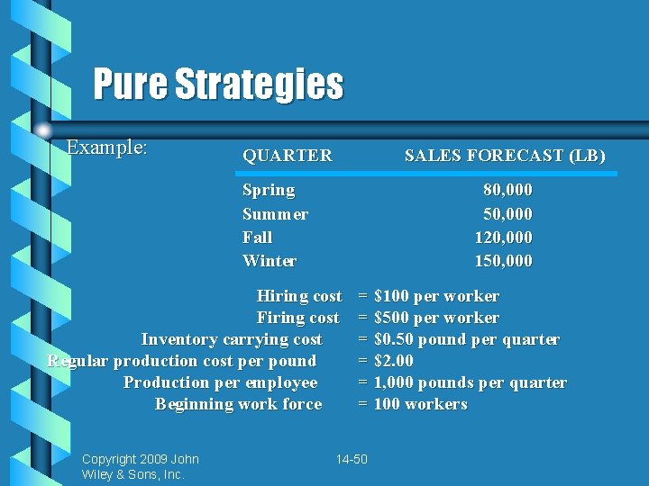
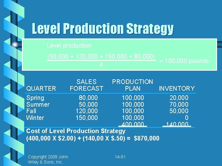
Pure Strategies Example: QUARTER SALES FORECAST (LB) Spring Summer Fall Winter 80, 000 50, 000 120, 000 150, 000 Hiring cost Firing cost Inventory carrying cost Regular production cost per pound Production per employee Beginning work force Copyright 2009 John Wiley & Sons, Inc. = $100 per worker = $500 per worker = $0. 50 pound per quarter = $2. 00 = 1, 000 pounds per quarter = 100 workers 14 -50

Level Production Strategy Level production (50, 000 + 120, 000 + 150, 000 + 80, 000) = 100, 000 pounds 4 QUARTER Spring Summer Fall Winter SALES FORECAST PRODUCTION PLAN INVENTORY 100, 000 400, 000 Cost of Level Production Strategy (400, 000 X $2. 00) + (140, 00 X $. 50) = $870, 000 Copyright 2009 John Wiley & Sons, Inc. 80, 000 50, 000 120, 000 150, 000 14 -51 20, 000 70, 000 50, 000 0 140, 000

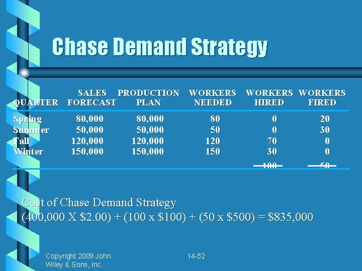
Chase Demand Strategy QUARTER Spring Summer Fall Winter SALES PRODUCTION FORECAST PLAN 80, 000 50, 000 120, 000 150, 000 WORKERS NEEDED HIRED FIRED 80 50 120 150 0 0 70 30 100 Cost of Chase Demand Strategy (400, 000 X $2. 00) + (100 x $100) + (50 x $500) = $835, 000 Copyright 2009 John Wiley & Sons, Inc. 14 -52 20 30 0 0 50

Chapter 9 – Project Management

Why has Project Management become so in-vogue? b Diversity of new products and product markets b Shorter life span of products b Rapid technological changes

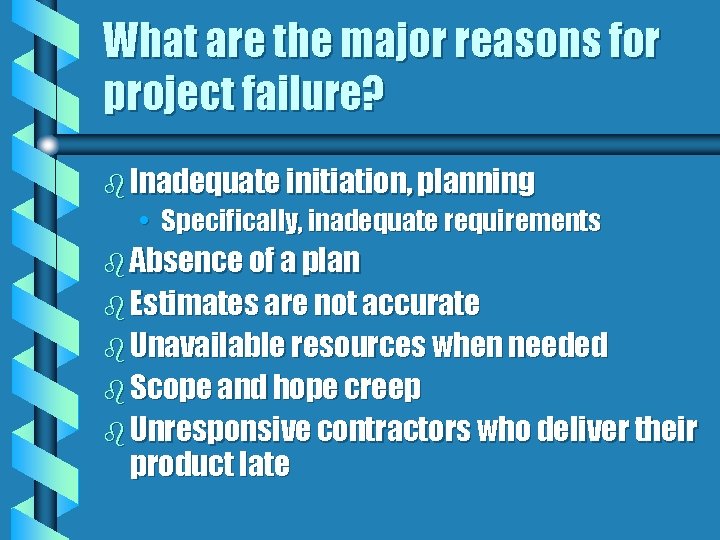
What are the major reasons for project failure? b Inadequate initiation, planning • Specifically, inadequate requirements b Absence of a plan b Estimates are not accurate b Unavailable resources when needed b Scope and hope creep b Unresponsive contractors who deliver their product late

What are the four phases of the project lifecycle? b Initiating b Planning b Executing b Closing b One other: Monitoring and Control

In which of these phases is a WBS started? b Planning • First 3 levels

The main purpose of a project plan is ____ b acquire resources bguide project execution. b meet standards expectations. b reduce risk.

The most important output of project execution is b. Work products b Not---change requests b Not—the WBS

The Principle… b That work tends to fill up the time allotted to it is known as…. .

An activity has probabilistic completion times of 20, 50 and 80 for the optimistic, most likely and pessimistic durations. What is the average time (duration) assuming a beta distribution? b 30 b 40 b 50 b 60 b 70

For each chapter…. b Skim the chapter b Examine the SUMMARY and the SUMMARY OF KEY TERMS SECTIONS at the end of each chapter

Chapter 2: Quality Management b Know the four operation types b Know the three types of make-tob Know the four dimensions of competition b What does DMAIC stand for?

Chapter 3: Quality Management b Name three quality gurus b Describe the relationship between TQM and continuous improvement b Understand the costs of quality b What is the relationship between quality and productivity? • Remember the yield formula? ?

Chapter 4: Statistical Quality Control b Know p-charts, c-charts, xbar-charts, rbar- charts b Which of these are used for attributes, which for variables? b Will not test you on AOQ, LTPD • {old antiquated concepts}

Chapter 6: Processes and Technologies Quality Function Deployment House of Quality

Chapter 6, Cont’d: Process Planning, Analysis… b Process analysis, flowcharts • SYMBOLS: Operation, Inspect, Transport, Delay, Storage b Flexible Manufacturing Sys, Robotics b IT: Ex. NETWORK Systems, Decision Support Systems b CIM

Reengineering design principles b Eliminate handoffs b Organize around outputs b Capture information once at the source b Eliminate multiple external contact points b Simplify work

Chapter 10: Supply Chain Management b Logistics by any other name b IT Integration b The bane of SCM is ______?

Chapter 14: Sales & Operations Planning b. Three planning horizons b Long-range planning b Medium range planning—aggregate prod planning b Short-range planning

Chapter 16: Just-in-time and Lean Production b Name five approaches to leanness… b What does SMED mean? b How can small lots be made economically effective?

Chapter 15: Enterprise Resource Planning b ERP Implementation is _____

Chapter 9: Project Management b Probabilistic NETWORK—be able to find the mean and standard deviation when given an optimistic, most likely and pessimistic estimate b. BE able to calculate project duration, project variance for NETWORK project TASKS

Network diagrams, drawn by commercial software b. Do they use • Activity-on-Node, or • Activity-on-Arrow representations?

That’s all folks b {I enjoyed having you as a class}