Review for Exam II This exam will be

Review for Exam II This exam will be administered Thursday, April 7, 2016, usual time and place

Exam Format ® 75 multiple choice ® Closed-book ® Closed-notes ® Closed-neighbor ® BRING---pencil, calculator, orange scantron sheet

Exam details ® Thursday, April 7, 2016 ® Will start the exam at 8: 00 a. m.

Exam Coverage ® Chs. 10, 11, 13, second half of 15 ® Supplements to chs. 11, 13, 14 LP problems in the supplement to Chapter 14, but not the content of Chapter 14—will cover that later. Will NOT Cover Ch. 12 (FORECASTING) You will, however, see the concept of collaborative planning, forecasting and replenishment on this exam—Ch. 11

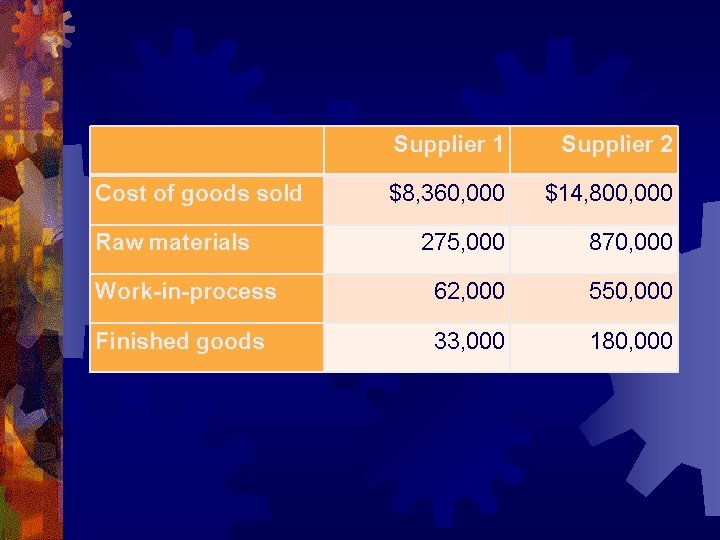
Supplier 1 Supplier 2 $8, 360, 000 $14, 800, 000 275, 000 870, 000 Work-in-process 62, 000 550, 000 Finished goods 33, 000 180, 000 Cost of goods sold Raw materials

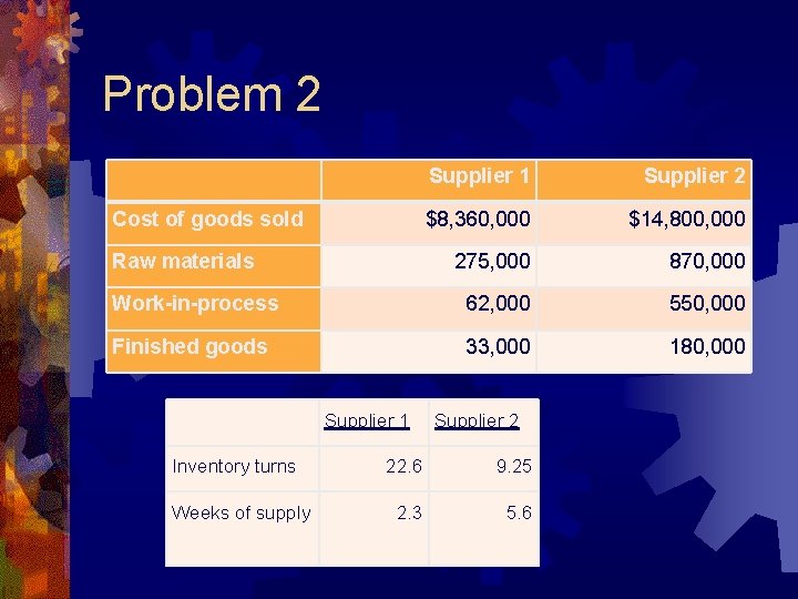
Problem 2 Supplier 1 Supplier 2 $8, 360, 000 $14, 800, 000 275, 000 870, 000 Work-in-process 62, 000 550, 000 Finished goods 33, 000 180, 000 Cost of goods sold Raw materials Supplier 1 Inventory turns Weeks of supply Supplier 2 22. 6 9. 25 2. 3 5. 6

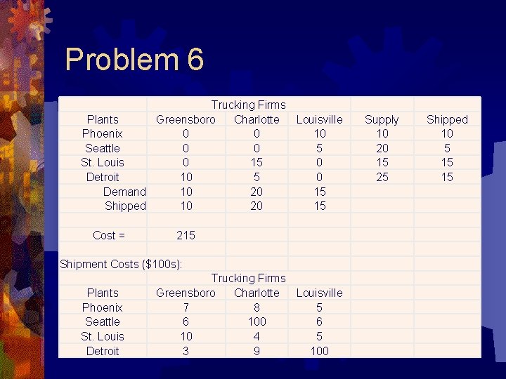
Problem 6 Trucking Firms Plants Greensboro Charlotte Louisville Phoenix 0 0 10 Seattle 0 0 5 St. Louis 0 15 0 Detroit 10 5 0 Demand 10 20 15 Shipped 10 20 15 Cost = 215 Shipment Costs ($100 s): Plants Phoenix Seattle St. Louis Detroit Trucking Firms Greensboro Charlotte Louisville 7 8 5 6 100 6 10 4 5 3 9 100 Supply 10 20 15 25 Shipped 10 5 15 15

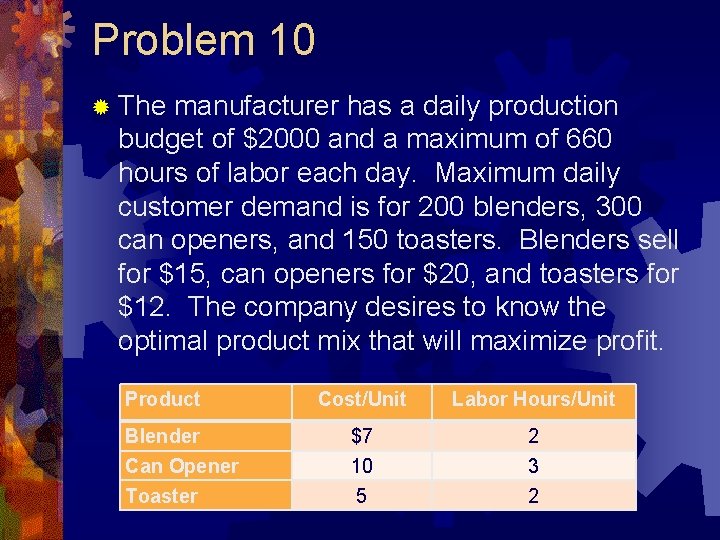
Problem 10 ® The manufacturer has a daily production budget of $2000 and a maximum of 660 hours of labor each day. Maximum daily customer demand is for 200 blenders, 300 can openers, and 150 toasters. Blenders sell for $15, can openers for $20, and toasters for $12. The company desires to know the optimal product mix that will maximize profit. Product Blender Can Opener Toaster Cost/Unit Labor Hours/Unit $7 10 5 2 3 2

Reduced Cost & Shadow Price ® Reduced Cost—the amount the associated obj. fcn. coefficient must be reduced by in order to get the associated decision variable to take on a value above zero ® Shadow Price—the amount the obj. fcn will change as a result of a unit change in a constraint right hand side.

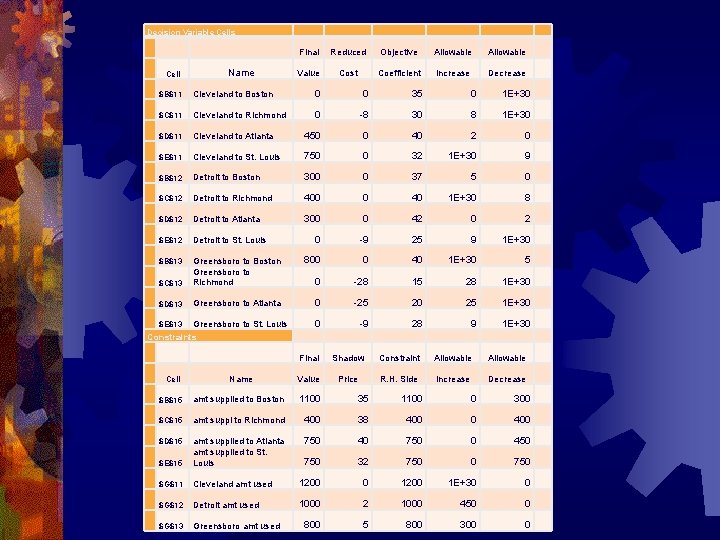
Decision Variable Cells Cell Name Final Reduced Objective Allowable Value Cost Coefficient Increase Decrease $B$11 Cleveland to Boston 0 0 35 0 1 E+30 $C$11 Cleveland to Richmond 0 -8 30 8 1 E+30 $D$11 Cleveland to Atlanta 450 0 40 2 0 $E$11 Cleveland to St. Louis 750 0 32 1 E+30 9 $B$12 Detroit to Boston 300 0 37 5 0 $C$12 Detroit to Richmond 400 0 40 1 E+30 8 $D$12 Detroit to Atlanta 300 0 42 0 2 $E$12 Detroit to St. Louis 0 -9 25 9 1 E+30 $B$13 800 0 40 1 E+30 5 $C$13 Greensboro to Boston Greensboro to Richmond 0 -28 15 28 1 E+30 $D$13 Greensboro to Atlanta 0 -25 20 25 1 E+30 0 -9 28 9 1 E+30 $E$13 Greensboro to St. Louis Constraints Cell Name Final Shadow Constraint Allowable Value Price R. H. Side Increase Decrease $B$15 amt supplied to Boston 1100 35 1100 0 300 $C$15 amt suppl to Richmond 400 38 400 0 400 $D$15 750 40 750 0 450 $E$15 amt supplied to Atlanta amt supplied to St. Louis 750 32 750 0 750 $G$11 Cleveland amt used 1200 0 1200 1 E+30 0 $G$12 Detroit amt used 1000 2 1000 450 0 $G$13 Greensboro amt used 800 5 800 300 0

Typical problems Embedded in the Multiple Choice ® Problems involving calculation of inventory turns and days of supply ® Production Scheduling Problem ® Transportation problem ® LP formulation problem ® Interpretation of LP SENSITIVITY output

Typical Problems Embedded within Multiple Choice ® Transshipment problem ® Linear programming formulation ® Simple EOQ Inventory problem ® EOQ with price-discounting

Chapter 15 – ERP ® Inventory for Dependent Demand will NOT be covered…. ® Exam coverage of this chapter starts on page 702 of the 8 th Edition

What were five motivations for transitioning from mainframes ® Absence of data integration ® 36 month backlogs at centralized MIS shops ® Idle CPU cycles on desktops ® Mainframes were expensive bottlenecks ® Support for Internet and thin clients ® Quicker, cheaper development times through REUSE

Every application software package consists of 1. 2. 3. 4. 5. Presentation management component Business logic management component Data management component All of the above 1 and 2 only

ERP ® Is software that organizes and manages a company’s business processes by sharing info across functional areas ® Large caps have been there and done that—transitioned to ERP ® Mid and small caps are getting there ® The road to implementation has been rough

More ERP ® Based on an N-tier distributed architecture ® Not on mainframe glasshouse

• Advantages of N-tier architecture ® Provides for data integration ® Better usage of MIPS on both PCs and servers ® Solves the 36 -month backlog of the centralized MIS shop ® Enables a better career path for the MIS professional

N-Tier distributed architecture ® Is decentralized or centralized, or some combination of these (which? ) ® Utilizes thick clients or thin clients (which? )

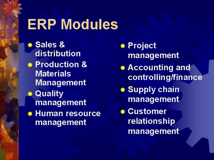
ERP Modules ® Sales & distribution ® Production & Materials Management ® Quality management ® Human resource management ® Project management ® Accounting and controlling/finance ® Supply chain management ® Customer relationship management

ERP Terms ® Best-of-breed ® Collaborative product commerce ® Customer relationship management ® Supply chain management ® XML

Distributed architectures solved these problems ® Data resides behind a single database engine

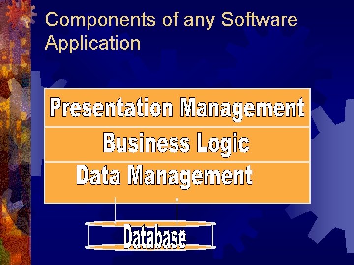
Components of any Software Application

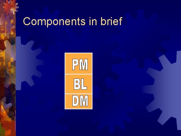
Components in brief

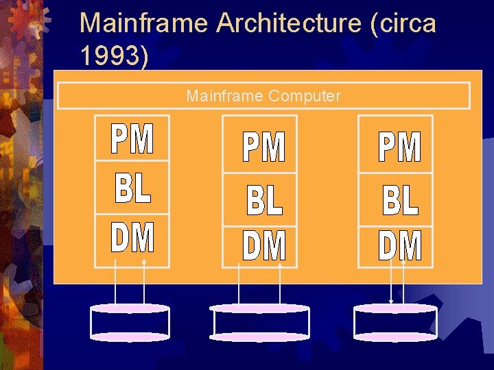
Mainframe Architecture (circa 1993) Mainframe Computer

Problems with Mainframe Architecture ® Absence of data integration, resulting in little enterprise visibility ® The applications are maintainable only by the centralized MIS shop, which is overloaded, resulting in 36 month lead times to get revisions effected ® Every application had to be built from scratch, line-by-line, resulting in large cost and long lead times to create new applications

More problems with Mainframe Architecture ® No reuse was possible ® These mainframe apps were accessed on networked PC’s via IBM 3278 terminal emulation software that was completely incompatible with the windows GUI applications—meaning no cut and paste ® Mainframes were computational bottlenecks ® Desktop PCs sat idle 99% of the time

Modern solution of today: NTIER DISTRIBUTED ARCHITECTURE ® This is a distributed architecture like client/server, but now the application is distributed across three or more computing boxes on the network

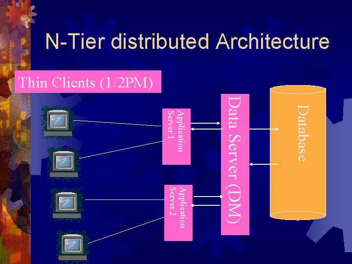
N-Tier distributed Architecture Thin Clients (1/2 PM) Database Application Server 2 Data Server (DM) Application Server 1

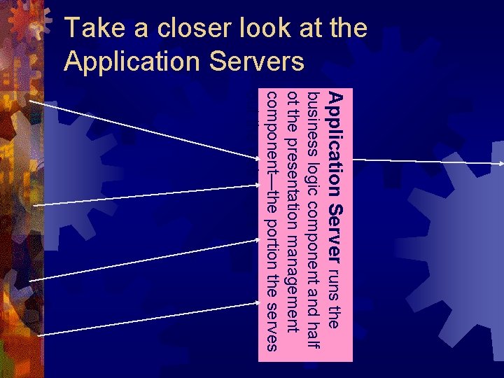
Take a closer look at the Application Servers Application Server runs the business logic component and half ot the presentation management component—the portion the serves out the web pages

Comments on N-Tier Distributed Architecture ® Clients are called ‘thin’ because the only thing running on them is the Internet Browser ® The IT professional doesn’t have to install anything on the client ® More re-use is possible—specifically that browser

Advantages of N-Tier Distributed Architecture ® Like Client/server, it accommodates enterprise visibility because the data are integrated ® Applications can be built rapidly because there is abundant reuse The DM module is reused ® Half of the PM component is reused ® There are reuse opportunities within the rest of the PM component and the BL component as well ®

More advantages of N-Tier ® IT professionals don’t have to be remotely loaned out to marketing, management, accounting and finance ® They can now be centrally located and managed where career paths will exist for them

Application Servers do Two things ® They serve out web pages upon request ® They do all of the business logic processing.

ERP Modules ® Finance/Accounting ® Sales Marketing ® Production/Materials Management ® Human Resources ® Supply Chain Management ® Customer Relation Management

These modules would be placed in a ® Thin client ® Data server ® Application server ® Mainframe WHICH? ?

ERP Implementation ® Analyze business processes ® Choose modules to implement ® Align level of sophistication ® Finalize delivery and access ® Link with External Partners

Customer Relationship Management ® CRM software plans and executes business processes that involve customer interaction, such as marketing, sales, fulfillment, and service (not manufacturing) ® CRM is focused on customers, not products

Collaborative Product Commerce ® Software concerned with new product design and development (possibly, across corporate boundaries), as well as product lifecycle management

Chapter 10 --Supply Chain Management ® Plants/warehouses/distribution/ information infrastructure ® Most of America’s non-bulk products get moved domestically by _____ (air, water, rail, truck, pipeline). ® What is COVISINT? ? ® What benefits accrue from SCM?

What’s new and exciting in SCM? ? ® Information Technology (specifically enterprise visibility) ® Has changed everything ® SCM Software modules within ERP systems ® I 2 Technologies ® Has reduced uncertainty Which has reduced _______ ® Which is a form of ________ ®

Inventory turns ® Calculated on an annual basis ® The more, the better ® Inputs: ® Cost of goods sold ® Average aggregate value of inventory

Average aggregate value of inventory ® Calculated by taking the product of the unit cost with the number of units and then summing these products for all inventory categories

YEARS OF SUPPLY ® YEARS OF SUPPLY = INVERSE OF INVENTORY TURNS PER YEAR

Days of supply ® Avg agg value of Inv*365/Ann cost of goods sold ® Or simply… 365/inventory turns ® Or simply 365 * years of supply

Manufacturing Inventory Types ® Raw materials inventory ® Work-in-process inventory ® Finished goods inventory

Supply Chain Management Terms ® ® ® ® ® Bullwhip effect Collaborative planning, forecasting and replenishment Continuous replenishment Core competencies Cross-docking E-business E-marketplaces E-procurement EDI Inventory turns Landed cost Logistics Order fulfillment RFID Sourcing Vendor-management inventory ® Warehouse management system ® ® ®

Chapter 13 – Inventory Management ® Inventory for Independent demand ® { Not manufacturing inventory, usually— more like retail inventory}

Carrying costs ® Rent ® Lighting/heating ® Security ® Interest (on borrowed capital tied up in inventory) ® Taxes ® Shrink/obsolescence/theft Can also be expressed as a % of product cost A rule of thumb is 30%

Ordering costs—costs related to Transportation Shipping Receiving Inspection

Shortage costs ® This is an opportunity cost ® Is ignored in the simple models you will be using, by assuming that there are no shortages

Back-order costs ® Will assume impatient customers who must have the product they wish to buy NOW. ® So back-ordering is not considered in the simple models we looked at

Continuous Inventory Systems ® Constant order amount, called the EOQ ® EOQ = Economic Order Quantity ® Fixed annual deterministic demand ® Minimizes ® Holding (carrying) costs ® Ordering costs ® Uses re-order point to determine when to order ® Time between orders is not fixed

EOQ models also have ® No shortages/back-ordering ® Constant lead time ® Instantaneous or finite replenishment ® Can take into consideration price discounting ® When doing so, three costs are minimized jointly: Ordering costs, holding costs and purchase costs taken over a year’s time

If the quantity ordered is less than the EOQ, then ® Ordering costs will be greater than holding (carrying) costs

Which gives you lowest holding cost? ® Instantaneous replenishment ® Finite (non-instantaneous) replenishment ® Quantity discounts ® WHICH OF THE ABOVE GIVES YOU LOWEST TOTAL ORDERING COST?

How do we calculate a reorder point? ® Lead time in days times the daily demand plus the safety stock ® Safety stock equals the service level (usually 3 for z) times the standard deviation of daily demand times the sq. rt. of lead time. ® (You will be given the formulas)

How do we calculate… ® Time between orders? ® Production ® Run days in a year / # of orders length ® EOQ rate or order quantity / daily Production

Safety Stocks and Service Levels ® Safety stock = Z value * std. dev. of daily demand * sqrt(lead time) A 95% service level means there is product to sell to customers 95% of the time. For 95% service level, use a Z value of 1. 65 ® For 99% service level, use Z value of 3

Inventory Terms ® ABC system ® Carrying costs ® Continuous inventory system ® Dependent demand ® EOQ ® Fixed-order quantity system ® Fixed time period system ® Capacity ® Independent demand ® Inventory ® In-process inventory ® Non-instantaneous receipt ® Order cycle ® Quantity discount ® Stockout ® Service level ® Efficiency

Simulation ® Two types— ® Continuous ® deterministic VENSIM is an example ® Discrete stochastic PROMODEL is an example ® SERVCEMODEL is an example ® ® Each of these two types differ by method of time advance

Time advance in continuous deterministic simulation ® Time is advanced in small, equidistant increments ® The simulation engine is really integrating differential equations

Time advance in discrete stochastic simulation ® Time is advanced from event to event ® The simulation engine maintains a stack of discrete events chronologically ordered in time, called an events calendar ® The next event to occur is popped off the stack and processed. ® The result of processing the event is that more events are generated and subsequently get saved on the events calendar

MONTE CARLO— ® The computer-generation of random numbers using an

Which simulation gestalt uses activities, events, entities and their attributes? ® Continuous deterministic? ® Discrete stochastic?

The Excel function RAND() generates… Normally-distributed random variates b. Gamma-distributed random variates c. Uniformly-distributed random numbers d. Exponentially-distributed random variates a.

To get a non-uniform random variate, we often start with A normal random variate b. A lognormal random variate c. A uniform random number d. A triangular random variate a.

In discrete/stochastic simulation, we are interested in a. b. c. d. e. Entity idleness Entity travel time Entity time in the system Resource utilization All of the above

In discrete/stochastic simulation, which of the following components has time duration? ® Events ® Activities ® Entities ® Resources ® All of the above

Discrete/stochastic simulation is appropriate for which of the following three decision environments ® Decision Making (DM) under Certainty ® DM under risk and uncertainty ® DM under change and complexity

Math programming models, like the transportation and transshipment models we looked at, are appropriate for which decision making environment ® Decision Making (DM) under Certainty ® DM under risk and uncertainty ® DM under change and complexity