Review Constraining global isoprene emissions with GOME formaldehyde

Review: Constraining global isoprene emissions with GOME formaldehyde column measurements Shim et al. Luz Teresa Padró Wei-Chun Hsieh Zhijun Zhao

Isoprene lifetime ~ 1 - 2 hr n Dominant Volatile Organic Compound (VOC) globally n Play important role in oxidant chemistry in troposphere n Non-Methane Hydrogen Carbon n VOC’s possibility of climate change

Isoprene II n Biogenic emission: vegetation n Emissions are favored by: n n n Vegetation types Light intensity Temperature Leaf area index (LAI) Oxidizes with OH and O 3 to produce formaldehyde n OH oxidation occurs faster and has higher yield

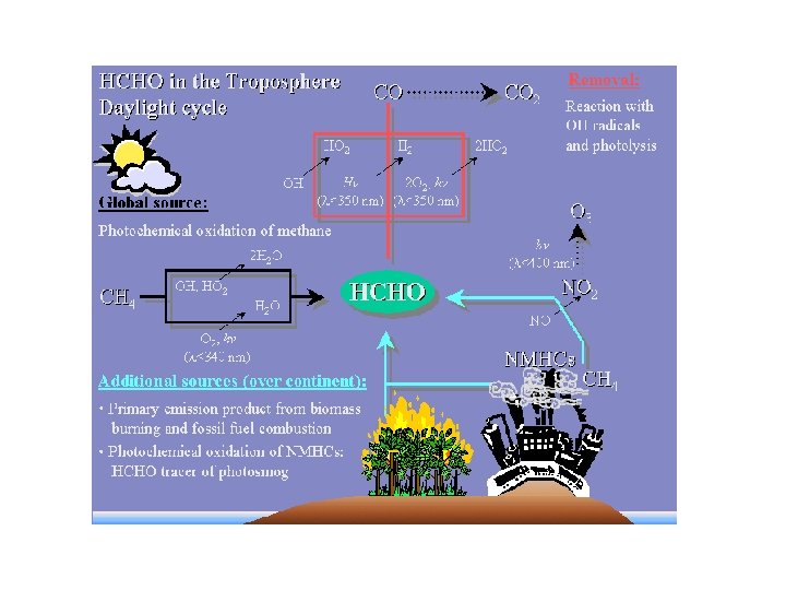
Isoprene Oxidation

Formaldehyde (HCHO) lifetime ~ 1. 5 days n n High-Yield Product of isoprene oxidation Source: methane Sink: photolysis and atmospheric OH Tracer for isoprene emissions

HCHO Column Observations n Obtained by the Global Ozone Monitoring Experiment (GOME) n n September 1996 – August 1997 Contributions to HCHO n n n 10 biogenic sources Biomass burning Industrial sources

Modeling Methods n A priori (forward model) n n A posteriori (inverse modeling) n n Uses global GEOS-CHEM chemical transport model Uses GOME measurements of formaldehyde to do inverse modeling to obtain isoprene emissions GEIA n Shows annual global isoprene distribution for 1990 inventory

GOME 1 HCHO Column Measurements and the Uncertainties n n n Affected by the South Atlantic Anomaly (SAA) do not include this region in inverse modeling AMFs (air mass factors) : covert slant columns to vertical columns AMF uncertainties due to uncertainties in UV albedo, vertical distribution of HCHO, and aerosols 1 Global Ozone Monitoring Experiment

Model n n n GEOS-CHEM Global 3 -D chemical transport model Comprehensive tropospheric O 3 -NOx-VOC chemical mechanism Oxidation mechanisms of 6 VOCs (ethane, propane, lumped >C 3 alkanes, lumped >C 2 alkenes, isoprene, and terpenes) 4 x 5 a maximum of 15 ecosystem types (area fraction, base emission) Seasonality (light intensity, temperature, and LAI)

Inverse Modeling n n n Only consider high signal-to-noise ratios in GOME measurements Criteria define regions for inverse modeling Daily GOME HCHO slant columns are > 4 d(1. 6*1016 molecules cm-2) Observations satisfy more than one season North America (eastern U. S. ), Europe (western Europe), East Asia, India, Southeast Asia, South America (Amazon), Africa, Australia

Inverse Modeling Regions

Inverse Modeling II n n n Using monthly GOME measurements with GEOS-CHEM as the forward model to estimate the source parameters of HCHO (state vector) Observation vector y and state vector x y=Kx+e

Global Distribution of the Vegetation Groups Tropical rain forest(V 1), grass/shrub(V 2), savanna(V 3), tropical seasonal forest& thorn woods(V 4), temperate mixed& temperate deciduous(V 5), agricultural lands(V 6), dry evergreen& crop/woods (warm) (V 7), regrowing woods(V 8), drought deciduous(V 9), the rest of ecosystems(V 10)

Result Analysis Isoprene Emission

Result Analysis Formaldehyde Column concentration

Result Analysis Regional isoprene emission (N. America, Europe, E. Aisa, India)

Result Analysis Regional isoprene emission (S. Asia, S. America, Africa, Australia)

Result Analysis

Effect of the Isoprene emission change On global OH concentration Decreased by 10. 8% 1. Convective transport 2. NOx reduce Emission over N. America

Effect of the Isoprene emission change On global NOx concentration Formation of PAN

Summary n n n 1. The a priori simulation greatly underestimates global HCHO columns and the a posteriori results show higher isoprene and biomass burning emission. 2. The a posteriori estimate a 50% larger annual isoprene emission than the a priori, decreasing global OH by 10. 8%. 3. The a posteriori global isoprene annual emission are higher at mid latitude and lower in tropics compared to the GEIA inventory.

Thank you!