Review Bayesian Networks Chapter 14 1 5 Basic

Review Bayesian Networks Chapter 14. 1 -5 • Basic concepts and vocabulary of Bayesian networks. – Nodes represent random variables. – Directed arcs represent (informally) direct influences. – Conditional probability tables, P( Xi | Parents(Xi) ). • Given a Bayesian network: – Write down the full joint distribution it represents. • Given a full joint distribution in factored form: – Draw the Bayesian network that represents it. • Given a variable ordering and background assertions of conditional independence among the variables: – Write down the factored form of the full joint distribution, as simplified by the conditional independence assertions. • Use the network to find answers to probability questions about it.

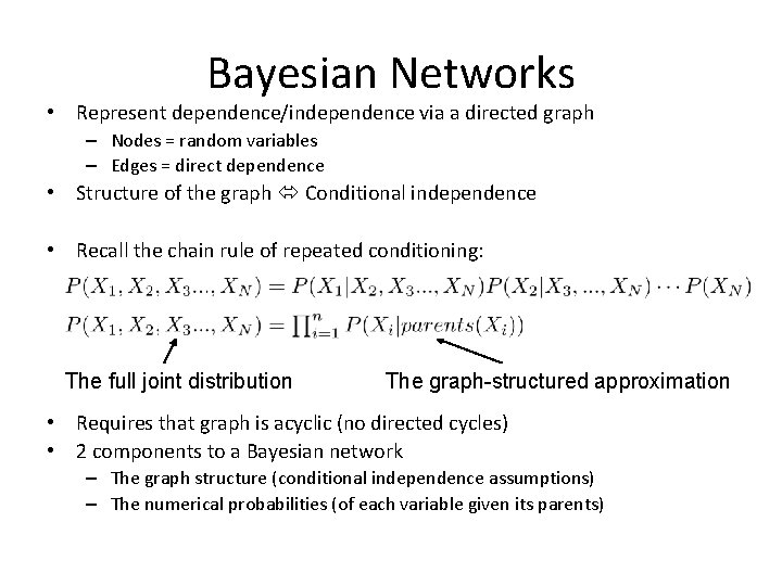
Bayesian Networks • Represent dependence/independence via a directed graph – Nodes = random variables – Edges = direct dependence • Structure of the graph Conditional independence • Recall the chain rule of repeated conditioning: The full joint distribution The graph-structured approximation • Requires that graph is acyclic (no directed cycles) • 2 components to a Bayesian network – The graph structure (conditional independence assumptions) – The numerical probabilities (of each variable given its parents)

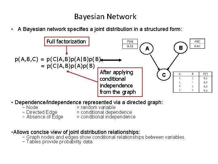
Bayesian Network • A Bayesian network specifies a joint distribution in a structured form: Full factorization B A p(A, B, C) = p(C|A, B)p(A|B)p(B) = p(C|A, B)p(A)p(B) After applying conditional independence from the graph C • Dependence/independence represented via a directed graph: − Node − Directed Edge − Absence of Edge = random variable = conditional dependence = conditional independence • Allows concise view of joint distribution relationships: − Graph nodes and edges show conditional relationships between variables. − Tables provide probability data.

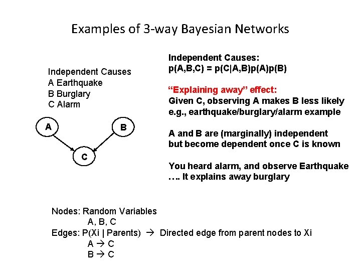
Examples of 3 -way Bayesian Networks Independent Causes A Earthquake B Burglary C Alarm A B C Independent Causes: p(A, B, C) = p(C|A, B)p(A)p(B) “Explaining away” effect: Given C, observing A makes B less likely e. g. , earthquake/burglary/alarm example A and B are (marginally) independent but become dependent once C is known You heard alarm, and observe Earthquake …. It explains away burglary Nodes: Random Variables A, B, C Edges: P(Xi | Parents) Directed edge from parent nodes to Xi A C B C

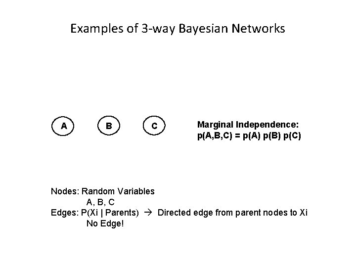
Examples of 3 -way Bayesian Networks A B C Marginal Independence: p(A, B, C) = p(A) p(B) p(C) Nodes: Random Variables A, B, C Edges: P(Xi | Parents) Directed edge from parent nodes to Xi No Edge!

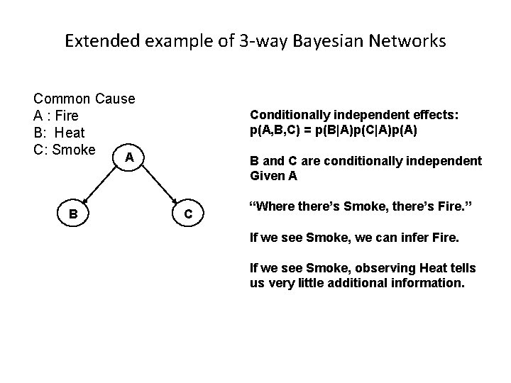
Extended example of 3 -way Bayesian Networks Common Cause A : Fire B: Heat C: Smoke Conditionally independent effects: p(A, B, C) = p(B|A)p(C|A)p(A) A B B and C are conditionally independent Given A C “Where there’s Smoke, there’s Fire. ” If we see Smoke, we can infer Fire. If we see Smoke, observing Heat tells us very little additional information.

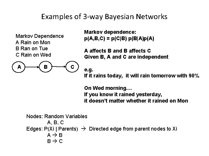
Examples of 3 -way Bayesian Networks Markov dependence: p(A, B, C) = p(C|B) p(B|A)p(A) Markov Dependence A Rain on Mon B Ran on Tue C Rain on Wed A B A affects B and B affects C Given B, A and C are independent C e. g. If it rains today, it will rain tomorrow with 90% On Wed morning… If you know it rained yesterday, it doesn’t matter whether it rained on Mon Nodes: Random Variables A, B, C Edges: P(Xi | Parents) Directed edge from parent nodes to Xi A B B C

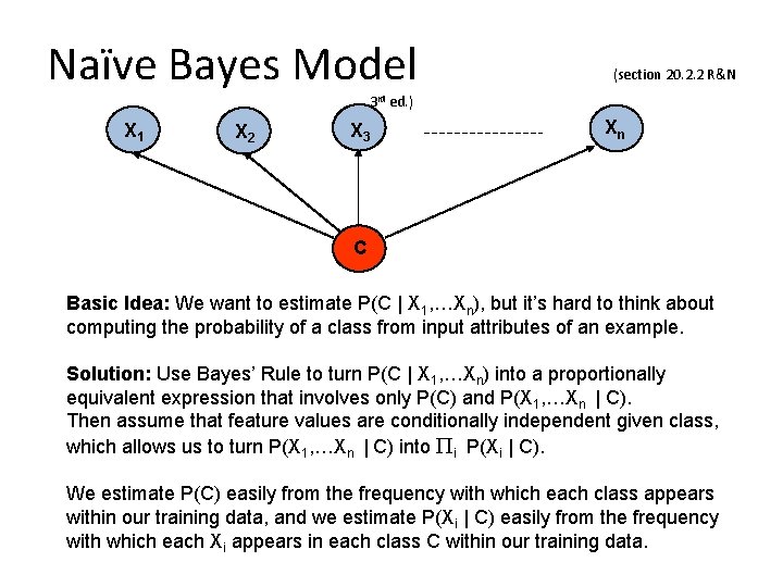
Naïve Bayes Model (section 20. 2. 2 R&N 3 rd ed. ) X 1 X 2 X 3 Xn C Basic Idea: We want to estimate P(C | X 1, …Xn), but it’s hard to think about computing the probability of a class from input attributes of an example. Solution: Use Bayes’ Rule to turn P(C | X 1, …Xn) into a proportionally equivalent expression that involves only P(C) and P(X 1, …Xn | C). Then assume that feature values are conditionally independent given class, which allows us to turn P(X 1, …Xn | C) into Pi P(Xi | C). We estimate P(C) easily from the frequency with which each class appears within our training data, and we estimate P(Xi | C) easily from the frequency with which each Xi appears in each class C within our training data.

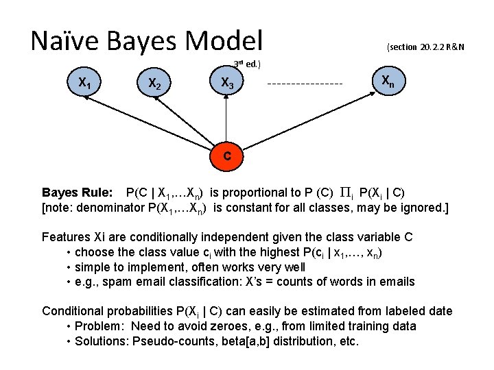
Naïve Bayes Model (section 20. 2. 2 R&N 3 rd ed. ) X 1 X 2 X 3 Xn C Bayes Rule: P(C | X 1, …Xn) is proportional to P (C) Pi P(Xi | C) [note: denominator P(X 1, …Xn) is constant for all classes, may be ignored. ] Features Xi are conditionally independent given the class variable C • choose the class value ci with the highest P(ci | x 1, …, xn) • simple to implement, often works very well • e. g. , spam email classification: X’s = counts of words in emails Conditional probabilities P(Xi | C) can easily be estimated from labeled date • Problem: Need to avoid zeroes, e. g. , from limited training data • Solutions: Pseudo-counts, beta[a, b] distribution, etc.

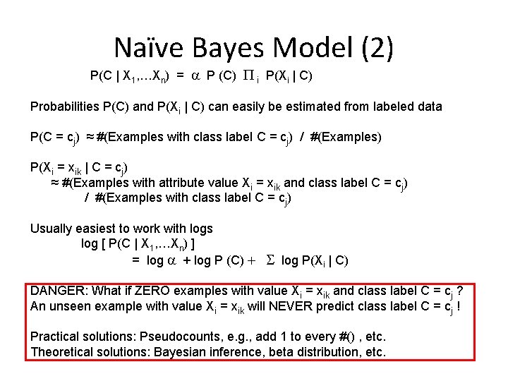
Naïve Bayes Model (2) P(C | X 1, …Xn) = a P (C) P i P(Xi | C) Probabilities P(C) and P(Xi | C) can easily be estimated from labeled data P(C = cj) ≈ #(Examples with class label C = cj) / #(Examples) P(Xi = xik | C = cj) ≈ #(Examples with attribute value Xi = xik and class label C = cj) / #(Examples with class label C = cj) Usually easiest to work with logs log [ P(C | X 1, …Xn) ] = log a + log P (C) + log P(Xi | C) DANGER: What if ZERO examples with value Xi = xik and class label C = cj ? An unseen example with value Xi = xik will NEVER predict class label C = cj ! Practical solutions: Pseudocounts, e. g. , add 1 to every #() , etc. Theoretical solutions: Bayesian inference, beta distribution, etc.

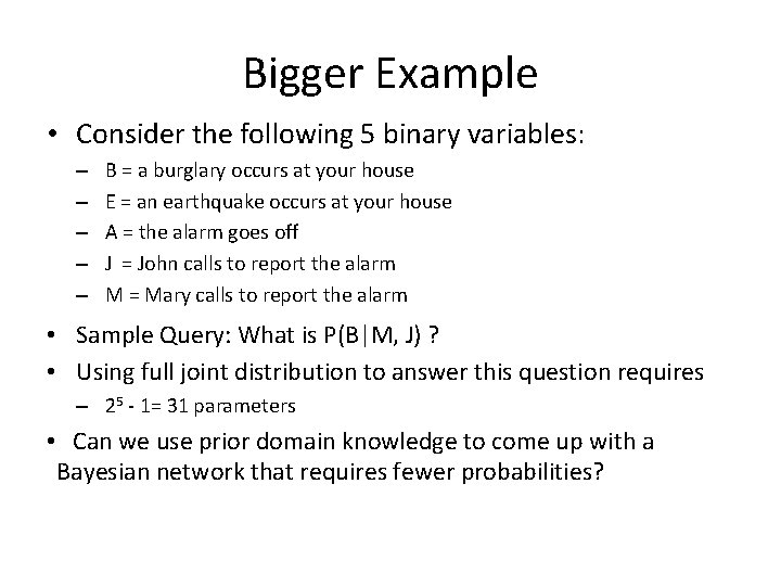
Bigger Example • Consider the following 5 binary variables: – – – B = a burglary occurs at your house E = an earthquake occurs at your house A = the alarm goes off J = John calls to report the alarm M = Mary calls to report the alarm • Sample Query: What is P(B|M, J) ? • Using full joint distribution to answer this question requires – 25 - 1= 31 parameters • Can we use prior domain knowledge to come up with a Bayesian network that requires fewer probabilities?

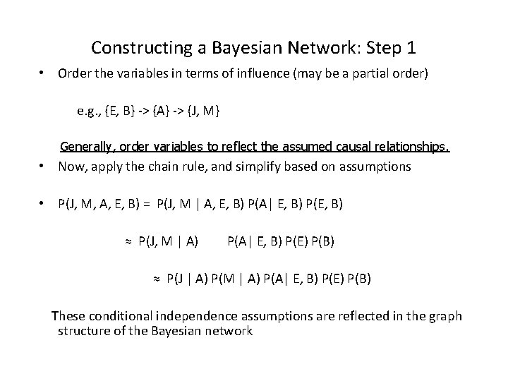
Constructing a Bayesian Network: Step 1 • Order the variables in terms of influence (may be a partial order) e. g. , {E, B} -> {A} -> {J, M} Generally, order variables to reflect the assumed causal relationships. • Now, apply the chain rule, and simplify based on assumptions • P(J, M, A, E, B) = P(J, M | A, E, B) P(A| E, B) P(E, B) ≈ P(J, M | A) P(A| E, B) P(E) P(B) ≈ P(J | A) P(M | A) P(A| E, B) P(E) P(B) These conditional independence assumptions are reflected in the graph structure of the Bayesian network

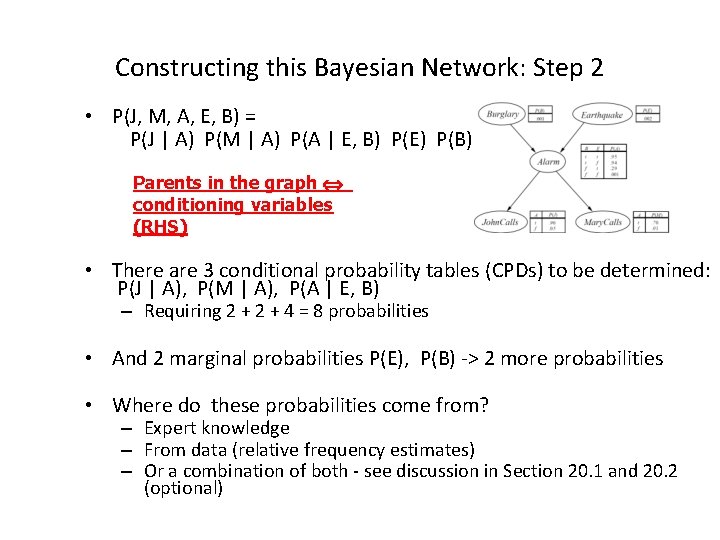
Constructing this Bayesian Network: Step 2 • P(J, M, A, E, B) = P(J | A) P(M | A) P(A | E, B) P(E) P(B) Parents in the graph conditioning variables (RHS) • There are 3 conditional probability tables (CPDs) to be determined: P(J | A), P(M | A), P(A | E, B) – Requiring 2 + 4 = 8 probabilities • And 2 marginal probabilities P(E), P(B) -> 2 more probabilities • Where do these probabilities come from? – Expert knowledge – From data (relative frequency estimates) – Or a combination of both - see discussion in Section 20. 1 and 20. 2 (optional)

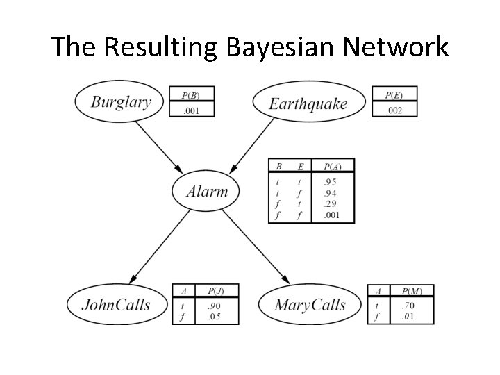
The Resulting Bayesian Network

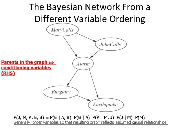
The Bayesian Network From a Different Variable Ordering Parents in the graph conditioning variables (RHS) P(J, M, A, E, B) = P(E | A, B) P(B | A) P(A | M, J) P(J | M) P(M) Generally, order variables so that resulting graph reflects assumed causal relationships.

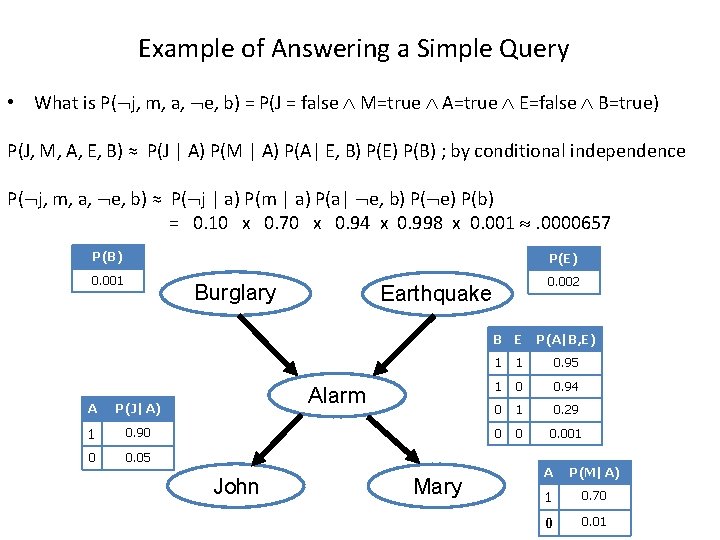
Example of Answering a Simple Query • What is P( j, m, a, e, b) = P(J = false M=true A=true E=false B=true) P(J, M, A, E, B) ≈ P(J | A) P(M | A) P(A| E, B) P(E) P(B) ; by conditional independence P( j, m, a, e, b) ≈ P( j | a) P(m | a) P(a| e, b) P( e) P(b) = 0. 10 x 0. 70 x 0. 94 x 0. 998 x 0. 001 . 0000657 P(B) P(E) 0. 001 0. 002 Burglary Earthquake B E A P(J|A) 1 0. 90 0 0. 05 Alarm John Mary P(A|B, E) 1 1 0. 95 1 0 0. 94 0 1 0. 29 0 0 0. 001 A P(M|A) 1 0. 70 0 0. 01

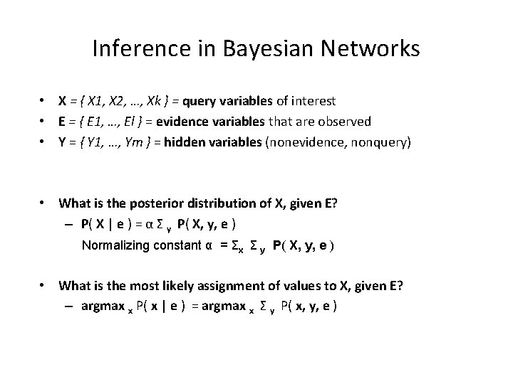
Inference in Bayesian Networks • X = { X 1, X 2, …, Xk } = query variables of interest • E = { E 1, …, El } = evidence variables that are observed • Y = { Y 1, …, Ym } = hidden variables (nonevidence, nonquery) • What is the posterior distribution of X, given E? – P( X | e ) = α Σ y P( X, y, e ) Normalizing constant α = Σx Σ y P( X, y, e ) • What is the most likely assignment of values to X, given E? – argmax x P( x | e ) = argmax x Σ y P( x, y, e )

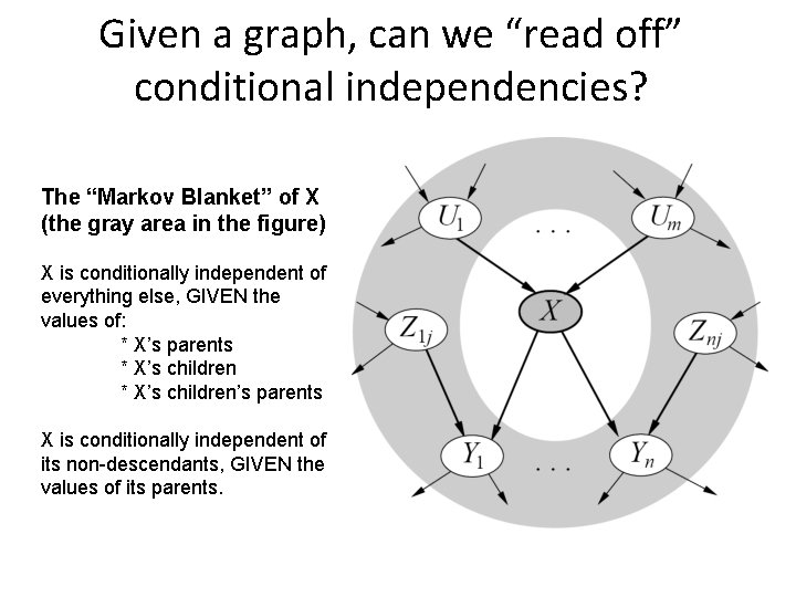
Given a graph, can we “read off” conditional independencies? The “Markov Blanket” of X (the gray area in the figure) X is conditionally independent of everything else, GIVEN the values of: * X’s parents * X’s children’s parents X is conditionally independent of its non-descendants, GIVEN the values of its parents.

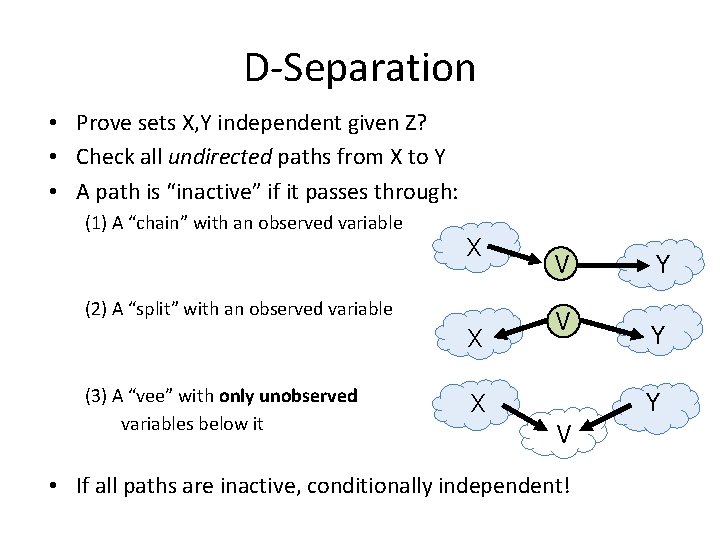
D-Separation • Prove sets X, Y independent given Z? • Check all undirected paths from X to Y • A path is “inactive” if it passes through: (1) A “chain” with an observed variable X (2) A “split” with an observed variable X (3) A “vee” with only unobserved variables below it V V Y Y Y X V • If all paths are inactive, conditionally independent!

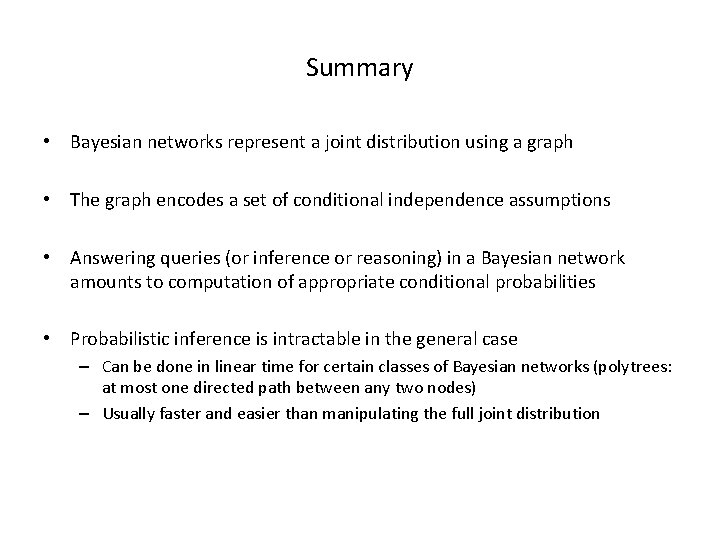
Summary • Bayesian networks represent a joint distribution using a graph • The graph encodes a set of conditional independence assumptions • Answering queries (or inference or reasoning) in a Bayesian network amounts to computation of appropriate conditional probabilities • Probabilistic inference is intractable in the general case – Can be done in linear time for certain classes of Bayesian networks (polytrees: at most one directed path between any two nodes) – Usually faster and easier than manipulating the full joint distribution