Review and Summary BoxJenkins models Stationary Time series

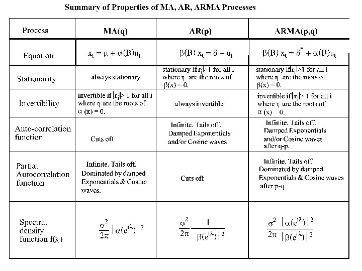
Review and Summary Box-Jenkins models Stationary Time series AR(p), MA(q), ARMA(p, q)

Models for Stationary Time Series.

The Moving Average Time series of order q, MA(q) is a Moving Average time series of order q. MA(q) if it satisfies the equation: where variance s 2. is a white noise time series with

The mean The autocovariance function for an MA(q) time series The autocorrelation function for an MA(q) time series

The Autoregressive Time series of order p, AR(p) {xt|t T} is called a Autoregressive time series of order p. AR(p) if it satisfies the equation: where {ut|t T} is a white noise time series with variance s 2.

The mean value of a stationary AR(p) series The Autocovariance function s(h) of a stationary AR(p) series Satisfies the equations:

The Autocorrelation function r(h) of a stationary AR(p) series Satisfies the equations: with for h > p and

or: where r 1, r 2, … , rp are the roots of the polynomial and c 1, c 2, … , cp are determined by using the starting values of the sequence r(h).

Stationarity AR(p) time series: consider the polynomial with roots r 1, r 2 , … , rp 1. then {xt|t T} is stationary if |ri| > 1 for all i. 2. If |ri| < 1 for at least one i then {xt|t T} exhibits deterministic behaviour. 3. If |ri| ≥ 1 and |ri| = 1 for at least one i then {xt|t T} exhibits non-stationary random behaviour.

The Mixed Autoregressive Moving Average Time Series of order p, ARMA(p, q) A Mixed Autoregressive- Moving Average time series - ARMA(p, q) series {xt: t T} satisfies the equation: where {ut|t T} is a white noise time series with variance s 2,

The mean value of a stationary ARMA(p, q) series Stationary of an ARMA(p, q) series Consider the polynomial with roots r 1, r 2 , … , rp 1. then {xt|t T} is stationary if |ri| > 1 for all i. 2. If |ri| < 1 for at least one i then {xt|t T} exhibits deterministic behaviour. 3. If |ri| ≥ 1 and |ri| = 1 for at least one i then {xt|t T} exhibits non-stationary random behaviour.

The autocovariance function s(h) satisfies: For h = 0, 1. … , q: for h > q:

h 0 -1 -2 -3 sux(h)

The partial auto correlation function at lag k is defined to be: Using Cramer’s Rule

A recursive formula for Fkk: Starting with F 11 = r 1 and

Spectral density function f(l)

Let {xt: t T} denote a time series with auto covariance function s(h) and let f(l) satisfy: then f(l) is called the spectral density function of the time series {xt: t T}

Linear Filters

Let {xt : t T} be any time series and suppose that the time series {yt : t T} is constructed as follows: : The time series {yt : t T} is said to be constructed from {xt : t T} by means of a Linear Filter. input xt Linear Filter as output yt

Spectral theory for Linear Filters if {yt : t T} is obtained from {xt : t T} by the linear filter:

Applications: The Moving Average Time series of order q, MA(q) since

The Autoregressive Time series of order p, AR(p) since

The ARMA(p, q) Time series of order p, q where {zt |t T} is a MA(q) time series. since

Three Important Forms of a Non-Stationary Time Series The Difference equation Form: b(B) xt = d + a(B)ut or xt = b 1 xt-1 + b 2 xt-2 +. . . +bpxt-p + d + ut +a 1 ut-1 + a 2 ut-2 +. . . +aqut-q

The Random Shock Form: xt = m+y(B)ut or xt = m + ut +y 1 ut-1 + y 2 ut-2 +y 3 ut-3 +. . . where y(B) = [b(B)]-1 a(B) = = I + y 1 B + y 2 B 2 +y 3 B 3 +. . . m = [b(B)]-1 d = d/(1 - b 2 -. . . - bp) and

The Inverted Form: p(B)xt = t + ut or xt = p 1 xt-1 + p 2 xt-2 +p 3 x 3+. . . + t + ut where p(B) = [a(B)]-1[b(B)] = I - p 1 B - p 2 B 2 - p 3 B 3 -. . .

Models for Non-Stationary Time Series The ARIMA(p, d, q) time series

An important fact: Most Non-stationary time series have changes that are stationary Recall the time series {xt : t T} defined by the following equation: xt = b 1 xt-1 + ut Then 1) if |b 1| < 1 then the time series {xt : t T} is a stationary time series. 2) if |b 1| = 1 then the time series {xt : t T} is a non stationary time series. 3) if |b 1| > 1 then the time series {xt : t T} is a deterministic time series in nature.

In fact if b 1 = 1 then this equation becomes: xt = xt-1 + ut This is the equation of a well known non stationary time series (called a Random Walk. ) Note: xt - xt-1 = (I - B)xt= Dxt = ut where D = I - B Thus by the simple transformation of computing first differences we can convert the time series {xt : t T} into a stationary time series.

Now consider the time series, {xt : t T}, defined by the equation: f(B)xt = d + a(B)ut where f(B) = I - f 1 B - f 2 B 2 -. . . - fp+d Bp+d. Let r 1, r 2, . . . , rp+d are the roots of the polynomial f(x) where: f(x) = 1 - f 1 x - f 2 x 2 -. . . - fp+dxp+d.

Then 1) if |ri| > 1 for i = 1, 2, . . . , p+d the time series {xt : t T} is a stationary time series. 2) if |ri| = 1 for at least one i (i = 1, 2, . . . , p) and |ri| > 1 for the remaining values of i then the time series {xt : t T} is a non stationary time series. 3) if |ri| < 1 for at least one i (i = 1, 2, . . . , p) then the time series {xt : t T} is a deterministic time series in nature.

Suppose that d roots of the polynomial f(x) are equal to unity then f(x) can be written: f(B) = (1 - b 1 x - b 2 x 2 -. . . - bpxp)(1 -x)d. and f(B) could be written: f(B) = (I - b 1 B - b 2 B 2 -. . . - bp. Bp)(I-B)d= b(B)Dd. In this case the equation for the time series becomes: f(B)xt = d + a(B)ut or b(B)Dd xt = d + a(B)ut. .

Thus if we let wt = Ddxt then the equation for {wt : t T} becomes: b(B)wt = d + a(B)ut Since the roots of b(B) are all greater than 1 in absolute value then the time series {wt: t T} is a stationary ARMA(p, q) time series. The original time series , {xt : t T}, is called an ARIMA(p, d, q) time series or Integrated Moving Average Autoregressive time series. The reason for this terminology is that in the case that d = 1 then {xt: t T} can be expressed in terms of {wt: t T} as follows: xt = D-1 wt = (I - B)-1 wt = (I + B 2 + B 3 + B 4+. . . )wt = wt + wt-1 + wt-2 + wt-3 + wt-4+. . .

Comments: 1. The operator f(B) =b(B)Dd is called the generalized autoregressive operator. 2. The operator b(B) is called the autoregressive operator. 3. The operator a(B) is called moving average operator. 4. If d = 0 then t the process is stationary and the level of the process is constant. 5. If d = 1 then the level of the process is randomly changing. 6. If d = 2 thern the slope of the process is randomly changing.

b(B)xt = d + a(B)ut

b(B)Dxt = d + a(B)ut

b(B)D 2 xt = d + a(B)ut

Forecasting for ARIMA(p, d, q) Time Series

Consider the m+n random variables x 1, x 2, . . . , xm, y 1, y 2, . . . , yn with joint density function f(x 1, x 2, . . . , xm, y 1, y 2, . . . , yn) = f(x, y) where x = (x 1, x 2, . . . , xm) and y = (y 1, y 2, . . . , yn).

Then the conditional density of x = (x 1, x 2, . . . , xm) given y = (y 1, y 2, . . . , yn) is defined to be:

In addition the conditional expectation of g(x) = g(x 1, x 2, . . . , xm) given y = (y 1, y 2, . . . , yn) is defined to be:

Prediction

Again consider the m+n random variables x 1, . . . , xm, y 1, . . . , yn. Suppose we are interested in predicting g(x 1, . . . , xm) = g(x) given y = (y 1, y 2, . . . , yn). Let t(y 1, y 2, . . . , yn) = t(y) denote any predictor of g(x 1, x 2, . . . , xm) = g(x) given the information in the observations y = (y 1, y 2, . . . , yn). Then the Mean square error of t(y) in predicting g(x) using t(y) is defined to be MSE[t(y)] = E[{t(y)-g(x)}2 |y]

It can be shown that the choice of t(y) that minimizes MSE[t(y)] is t(y) = E[g(x) |y]. Proof: Let v(t) = E{[t-g(x)]2 |y } = E[t 2 -2 tg(x)+g 2(x) |y] = t 2 -2 t. E[g(x)|y]+E[g 2(x) |y]. Then v'(t) = 2 t -2 E[g(x)|y] = 0 when t = E[g(x)|y].

Three Important Forms of a Non-Stationary Time Series The Difference equation Form: b(B)Ddxt = d + a(B)ut or f(B)xt = d + a(B)ut or xt = f 1 xt-1 + f 2 xt-2 +. . . +fp+dxt-p-d + ut +a 1 ut-1 + a 2 ut-2 +. . . +aqut-q

The Random Shock Form: xt = m(t) +y(B)ut or xt = m(t) + ut +y 1 ut-1 + y 2 ut-2 +y 3 ut-3 +. . . where y(B) = [f(B)]-1 a(B) = [b(B)Dd]-1 a(B) = I + y 1 B + y 2 B 2 +y 3 B 3 +. . . m = [b(B)]-1 d= d/(1 - b 2 -. . . - bp) and m(t) = D-dm

Note: Ddm(t) = m i. e. the dth order differences are constant. This implies that m(t) is a polynomial of degree d.

Consider The Difference equation Form: b(B)Ddxt = d + a(B)ut or f(B)xt = d + a(B)ut

Multiply both sides by f(B)-1 To get f(B)-1 f(B)xt = f(B)-1 d + f(B)-1 a(B)ut or xt = f(B)-1 d + f(B)-1 a(B)ut

The Inverted Form: p(B)xt = t + ut or xt = p 1 xt-1 + p 2 xt-2 +p 3 x 3+. . . + t + ut where p(B) = [a(B)]-1 f(B) = [a(B)]-1[b(B)Dd] = I - p 1 B - p 2 B 2 - p 3 B 3 -. . .

Again Consider The Difference equation Form: f(B)xt = d + a(B)ut Multiply both sides by a(B)-1 To get a(B)-1 f(B)xt = a(B)-1 d + a(B)-1 a(B)ut or p(B) xt = t + ut

Forecasting an ARIMA(p, d, q) Time Series • Let PT denote {…, x. T-2, x. T-1, x. T} = the “past” til time T. • Then the optimal forecast of x. T+l given PT is denoted by: • This forecast minimizes the mean square error

Three different forms of the forecast 1. Random Shock Form 2. Inverted Form 3. Difference Equation Form Note:

Random Shock Form of the forecast Recall xt = m(t) + ut +y 1 ut-1 + y 2 ut-2 +y 3 ut-3 +. . . or x. T+l = m(T + l) + u. T+l +y 1 u. T+l-1 + y 2 u. T+l-2 +y 3 u. T+l-3 +. . . Taking expectations of both sides and using

To compute this forecast we need to compute {…, u. T-2, u. T-1, u. T} from {…, x. T-2, x. T-1, x. T}. Note: xt = m(t) + ut +y 1 ut-1 + y 2 ut-2 +y 3 ut-3 +. . . Thus and Which can be calculated recursively

The Error in the forecast: The Mean Sqare Error in the Forecast Hence

Prediction Limits forecasts (1 – a)100% confidence limits for x. T+l

The Inverted Form: p(B)xt = t + ut or xt = p 1 xt-1 + p 2 xt-2 +p 3 x 3+. . . + t + ut where p(B) = [a(B)]-1 f(B) = [a(B)]-1[b(B)Dd] = I - p 1 B - p 2 B 2 - p 3 B 3 -. . .

The Inverted form of the forecast Note: xt = p 1 xt-1 + p 2 xt-2 +. . . + t + ut and for t = T+l x. T+l = p 1 x. T+l-1 + p 2 x. T+l-2 +. . . + t + u. T+l Taking conditional Expectations

The Difference equation form of the forecast x. T+l = f 1 x. T+l-1 + f 2 x. T+l-2 +. . . + fp+dx. T+l-p-d + u. T+l +a 1 u. T+l-1 + a 2 u. T+l-2 +. . . + aqu. T+l-q Taking conditional Expectations

Example: The Model: xt - xt-1 = b 1(xt-1 - xt-2) + ut + a 1 ut + a 2 ut or xt = (1 + b 1)xt-1 - b 1 xt-2 + ut + a 1 ut + a 2 ut or f(B)xt = b(B)(I-B)xt = a(B)ut where f(x) = 1 - (1 + b 1)x + b 1 x 2 = (1 - b 1 x)(1 -x) and a(x) = 1 + a 1 x + a 2 x 2.

The Random Shock form of the model: xt =y(B)ut where y(B) = [b(B)(I-B)]-1 a(B) = [y(B)]-1 a(B) i. e. y(B) [f(B)] = a(B). Thus (I + y 1 B + y 2 B 2 + y 3 B 3 + y 4 B 4 +. . . )(I - (1 + b 1)B + b 1 B 2) = I + a 1 B + a 2 B 2 Hence a 1 = y 1 - (1 + b 1) or y 1 = 1 + a 1 + b 1. a 2 = y 2 - y 1(1 + b 1) + b 1 or y 2 =y 1(1 + b 1) - b 1 + a 2. 0 = yh - yh-1(1 + b 1) + yh-2 b 1 or yh = yh-1(1 + b 1) - yh-2 b 1 for h ≥ 3.

The Inverted form of the model: p(B) xt = ut where p(B) = [a(B)]-1 b(B)(I-B) = [a(B)]-1 f(B) i. e. p(B) [a(B)] = f(B). Thus (I - p 1 B - p 2 B 2 - p 3 B 3 - p 4 B 4 -. . . )(I + a 1 B + a 2 B 2) = I - (1 + b 1)B + b 1 B 2 Hence -(1 + b 1) = a 1 - p 1 or p 1 = 1 + a 1 + b 1 = -p 2 - p 1 a 1 + a 2 or p 2 = -p 1 a 1 - b 1 + a 2. 0 = -ph - ph-1 a 1 - ph-2 a 2 or ph = -(ph-1 a 1 + ph-2 a 2) for h ≥ 3.

Now suppose that b 1 = 0. 80, a 1 = 0. 60 and a 2 = 0. 40 then the Random Shock Form coefficients and the Inverted Form coefficients can easily be computed and are tabled below: