Return Map Algorithm on StaggeredGrid FD AWP Code

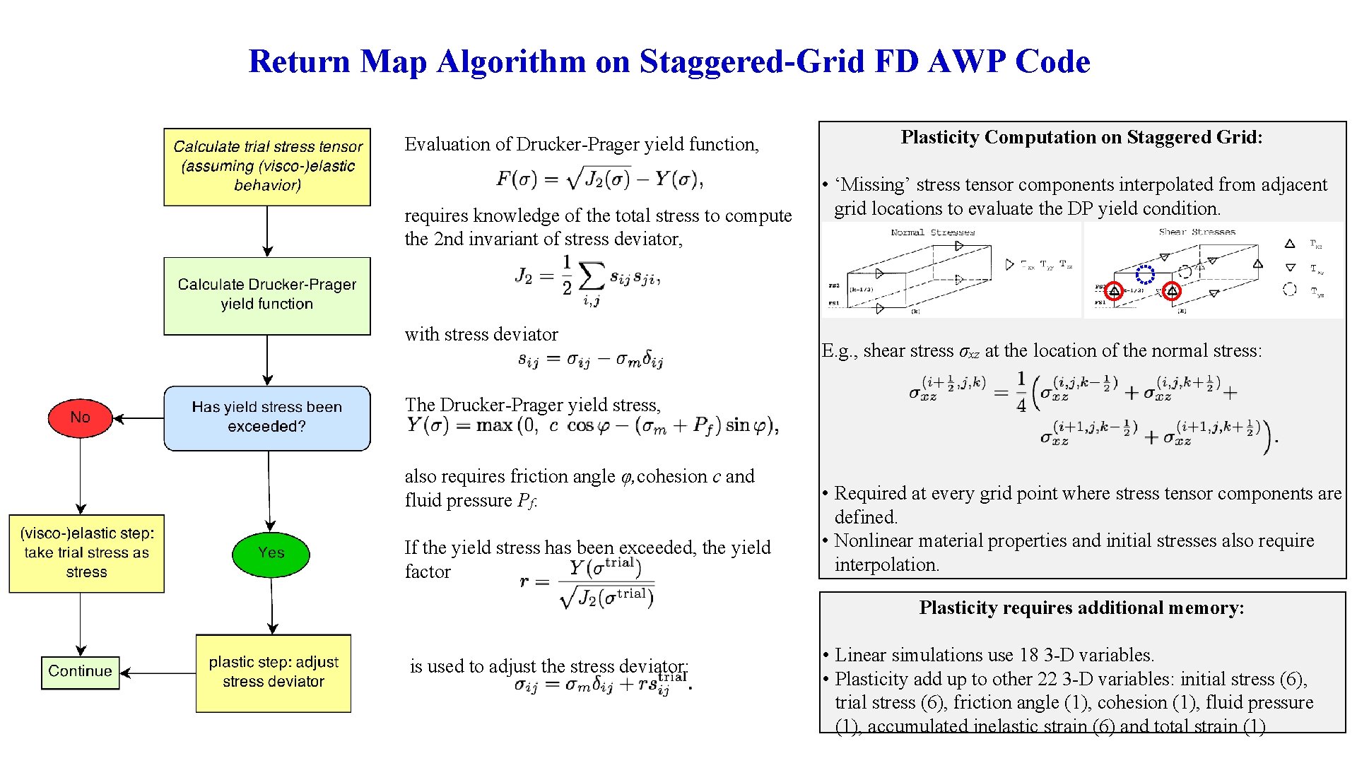
Return Map Algorithm on Staggered-Grid FD AWP Code Evaluation of Drucker-Prager yield function, requires knowledge of the total stress to compute the 2 nd invariant of stress deviator, with stress deviator Plasticity Computation on Staggered Grid: • ‘Missing’ stress tensor components interpolated from adjacent grid locations to evaluate the DP yield condition. E. g. , shear stress σxz at the location of the normal stress: The Drucker-Prager yield stress, also requires friction angle φ, cohesion c and fluid pressure Pf. If the yield stress has been exceeded, the yield factor • Required at every grid point where stress tensor components are defined. • Nonlinear material properties and initial stresses also require interpolation. Plasticity requires additional memory: is used to adjust the stress deviator: • Linear simulations use 18 3 -D variables. • Plasticity add up to other 22 3 -D variables: initial stress (6), trial stress (6), friction angle (1), cohesion (1), fluid pressure (1), accumulated inelastic strain (6) and total strain (1)

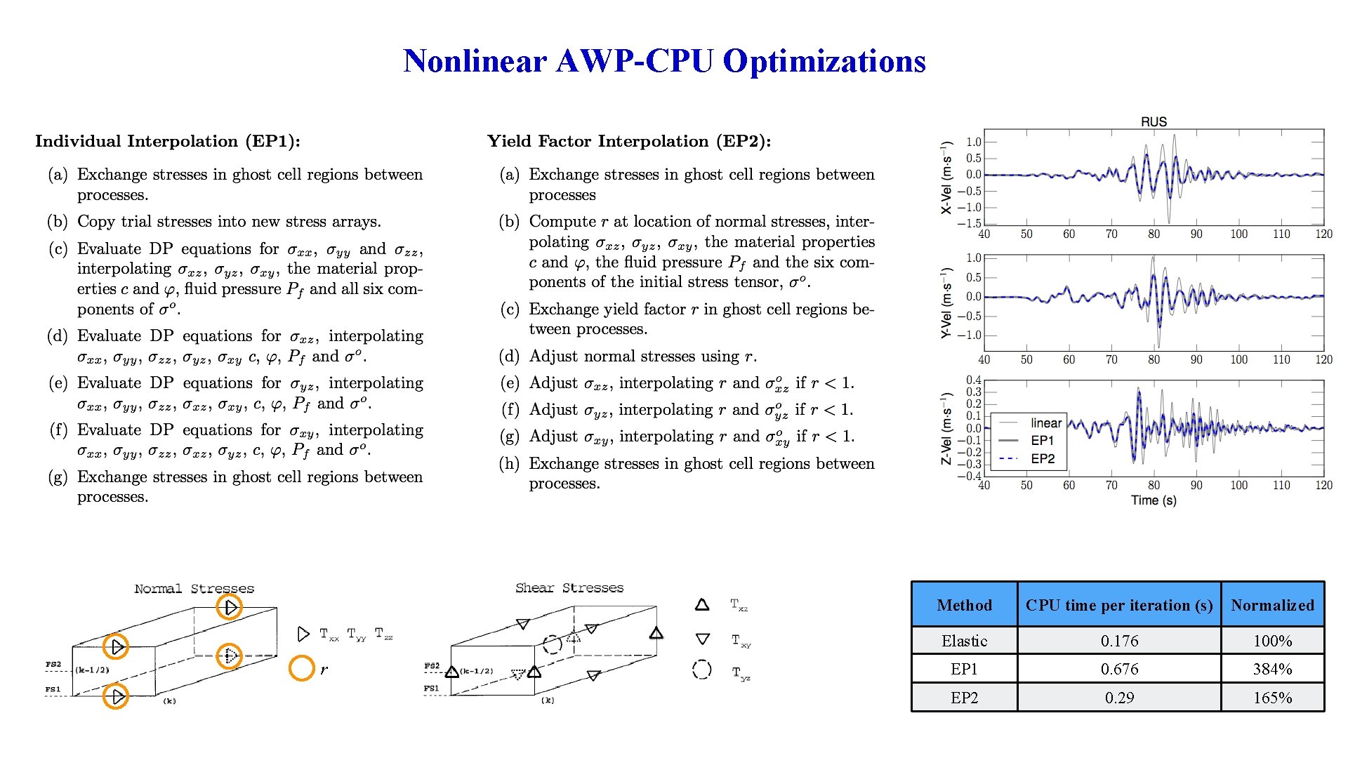
Nonlinear AWP-CPU Optimizations r Method CPU time per iteration (s) Normalized Elastic 0. 176 100% EP 1 0. 676 384% EP 2 0. 29 165%

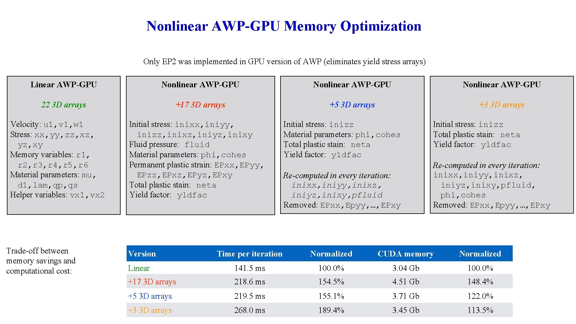
Nonlinear AWP-GPU Memory Optimization Only EP 2 was implemented in GPU version of AWP (eliminates yield stress arrays) Linear AWP-GPU Nonlinear AWP-GPU 22 3 D arrays +17 3 D arrays +5 3 D arrays +3 3 D arrays Velocity: u 1, v 1, w 1 Stress: xx, yy, zz, xz, yz, xy Memory variables: r 1, r 2, r 3, r 4, r 5, r 6 Material parameters: mu, d 1, lam, qp, qs Helper variables: vx 1, vx 2 Trade-off between memory savings and computational cost: Initial stress: inixx, iniyy, inizz, inixz, iniyz, inixy Fluid pressure: fluid Material parameters: phi, cohes Permanent plastic strain: EPxx, EPyy, EPzz, EPxz, EPyz, EPxy Total plastic stain: neta Yield factor: yldfac Version Initial stress: inizz Material parameters: phi, cohes Total plastic stain: neta Yield factor: yldfac Re-computed in every iteration: inixx, iniyy, inixz, iniyz, inixy, pfluid Removed: EPxx, Epyy, …, EPxy Initial stress: inizz Total plastic stain: neta Yield factor: yldfac Re-computed in every iteration: inixx, iniyy, inixz, iniyz, inixy, pfluid, phi, cohes Removed: EPxx, Epyy, …, EPxy Time per iteration Normalized CUDA memory Normalized Linear 141. 5 ms 100. 0% 3. 04 Gb 100. 0% +17 3 D arrays 218. 6 ms 154. 5% 4. 51 Gb 148. 4% +5 3 D arrays 219. 5 ms 155. 1% 3. 71 Gb 122. 0% +3 3 D arrays 268. 0 ms 189. 4% 3. 45 Gb 113. 5%

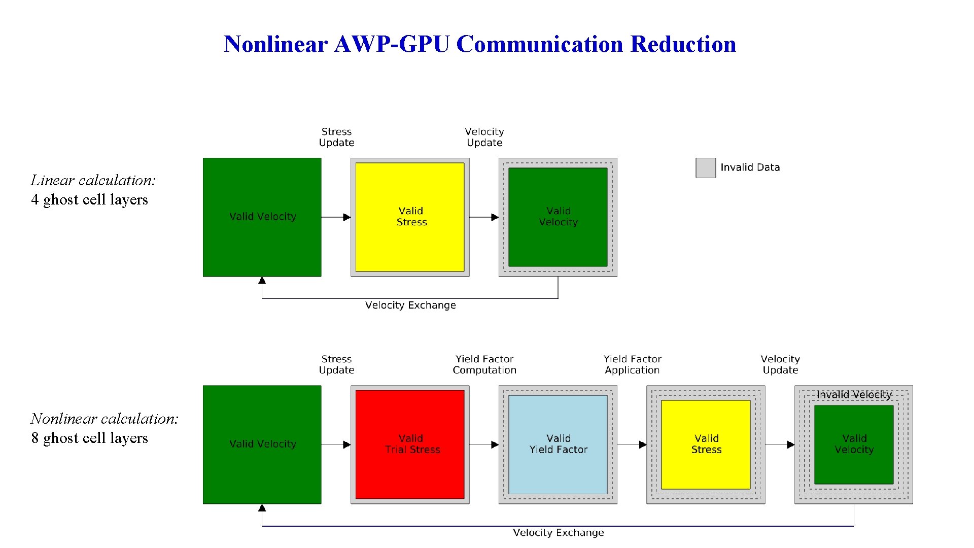
Nonlinear AWP-GPU Communication Reduction Linear calculation: 4 ghost cell layers Nonlinear calculation: 8 ghost cell layers

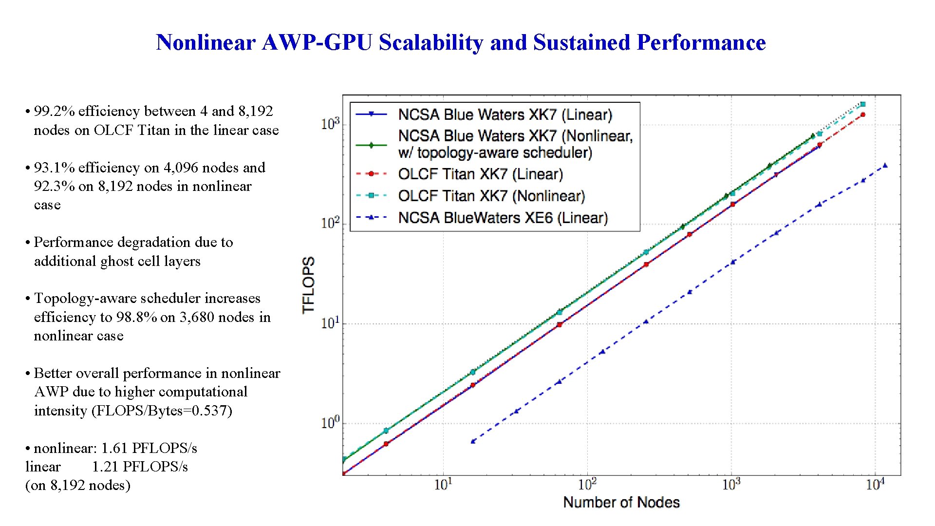
Nonlinear AWP-GPU Scalability and Sustained Performance • 99. 2% efficiency between 4 and 8, 192 nodes on OLCF Titan in the linear case • 93. 1% efficiency on 4, 096 nodes and 92. 3% on 8, 192 nodes in nonlinear case • Performance degradation due to additional ghost cell layers • Topology-aware scheduler increases efficiency to 98. 8% on 3, 680 nodes in nonlinear case • Better overall performance in nonlinear AWP due to higher computational intensity (FLOPS/Bytes=0. 537) • nonlinear: 1. 61 PFLOPS/s linear 1. 21 PFLOPS/s (on 8, 192 nodes)

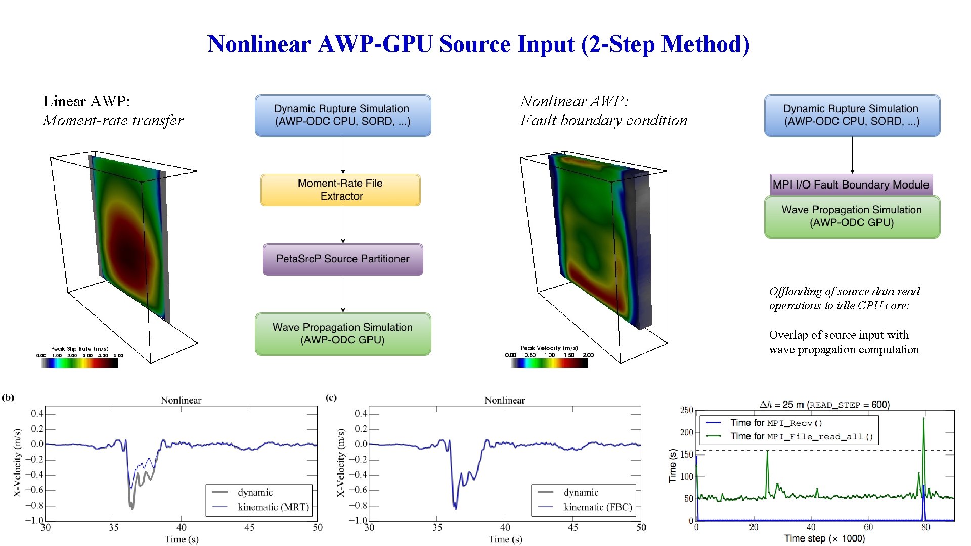
Nonlinear AWP-GPU Source Input (2 -Step Method) Linear AWP: Moment-rate transfer Nonlinear AWP: Fault boundary condition Offloading of source data read operations to idle CPU core: Overlap of source input with wave propagation computation

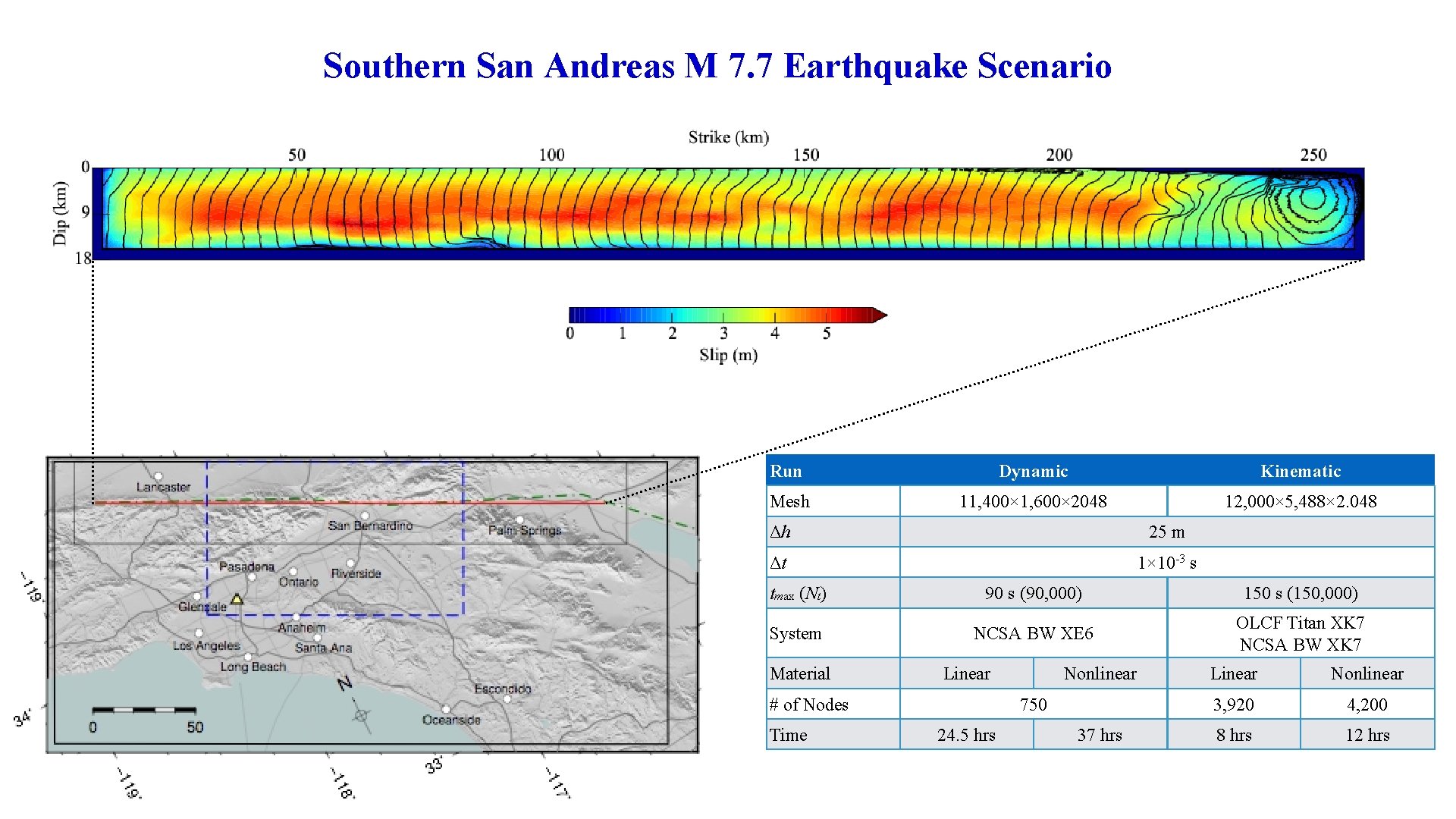
Southern San Andreas M 7. 7 Earthquake Scenario Run Dynamic Kinematic Mesh 11, 400× 1, 600× 2048 12, 000× 5, 488× 2. 048 Δh 25 m Δt 1× 10 -3 s tmax (Nt) 90 s (90, 000) 150 s (150, 000) System NCSA BW XE 6 OLCF Titan XK 7 NCSA BW XK 7 Material Linear # of Nodes Time Nonlinear 750 24. 5 hrs 37 hrs Linear Nonlinear 3, 920 4, 200 8 hrs 12 hrs

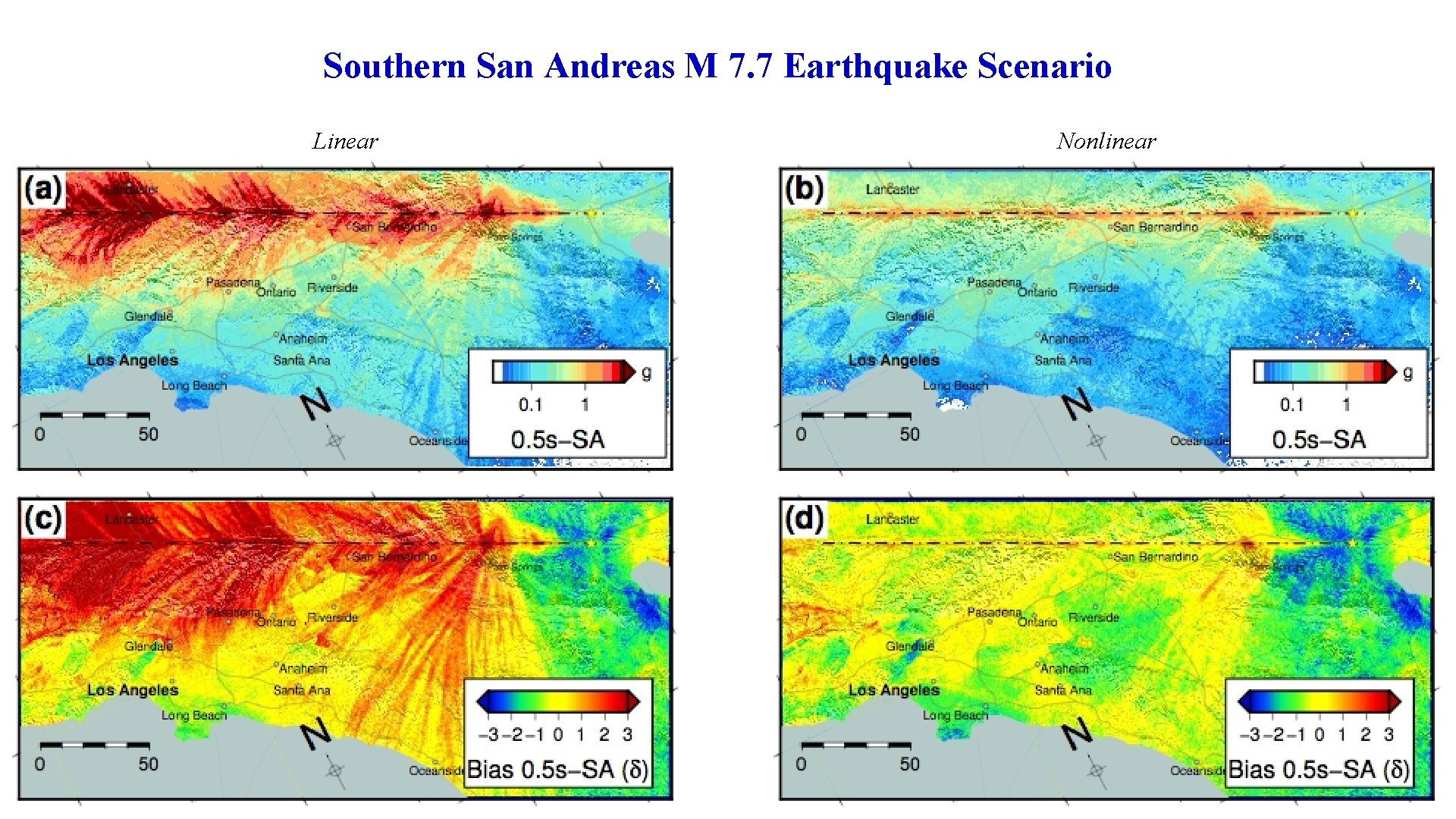
Southern San Andreas M 7. 7 Earthquake Scenario Linear Nonlinear