Restricted Boltzmann Machine and Deep Belief Net Wanli

Restricted Boltzmann Machine and Deep Belief Net Wanli Ouyang wlouyang@ee. cuhk. edu. hk Animation is available for illustration 1

Outline • Short introduction on deep learning • Short introduction on statistical models and Graphical model • Restricted Boltzmann Machine (RBM) and Contrastive divergence • Deep belief net (DBN) RBM and DBN are statistical models Deep belief net is trained using RBM and CD Deep belief net is an unsupervised training algorithm for deep neural network 2

Good learning resources • Webpages: – Geoffrey E. Hinton’s readings (with source code available for DBN) http: //www. cs. toronto. edu/~hinton/csc 2515/deeprefs. html – Notes on Deep Belief Networks http: //www. quantumg. net/dbns. php – MLSS Tutorial, October 2010, ANU Canberra, Marcus Frean http: //videolectures. net/mlss 2010 au_frean_deepbeliefnets/ – Deep Learning Tutorials http: //deeplearning. net/tutorial/ – Hinton’s Tutorial, http: //videolectures. net/mlss 09 uk_hinton_dbn/ – Fergus’s Tutorial, http: //cs. nyu. edu/~fergus/presentations/nips 2013_final. pdf – CUHK MMlab project : http: //mmlab. ie. cuhk. edu. hk/project_deep_learning. html • People: – – – – Geoffrey E. Hinton’s http: //www. cs. toronto. edu/~hinton Andrew Ng http: //www. cs. stanford. edu/people/ang/index. html Ruslan Salakhutdinov http: //www. utstat. toronto. edu/~rsalakhu/ Yee-Whye Teh http: //www. gatsby. ucl. ac. uk/~ywteh/ Yoshua Bengio www. iro. umontreal. ca/~bengioy Yann Le. Cun http: //yann. lecun. com/ Marcus Frean http: //ecs. victoria. ac. nz/Main/Marcus. Frean Rob Fergus http: //cs. nyu. edu/~fergus/pmwiki. php • Acknowledgement – Many materials in this ppt are from these papers, tutorials, etc (especially Hinton and Frean’s). Sorry for not listing them in full detail. 3 Dumitru Erhan, Aaron Courville, Yoshua Bengio. Understanding Representations Learned in Deep Architectures. Technical Report.

Neural network Back propagation 1986 Deep belief net Science Speech 2006 2011 2012 deep learning results • • Unsupervised & Layer-wised pre-training Loose tie with biological systems • SVM … …Rank Name Error Description • • Better designs for modeling and training Shallow model • Solve general learning problems • Boosting rate (normalization, nonlinearity, dropout) • Specific methods for specific tasks … … • Tied with biological system But it is given up… • Decision tree – Hand crafted features (GMM-HMM, SIFT, LBP, HOG) 1 U. Toronto 0. 15315 Deep learning • Feature learning … … 2 Hard to train • KNN U. Tokyo 0. 26172 Hand-crafted • • New development of computer architectures • –Insufficient computational resources • …… … 3 U. Oxford. GPU 0. 26979 features and • –Small training sets learning models. Multi-core computer systems 4 Xerox/INRIA 0. 27058 • Does not work well Bottleneck. • Large scale databases Object recognition over 1, 000 images and 1, 000 categories How Many Computers to Identify a Cat? 16000 CPU cores Kruger et al. TPAMI’ 13 (2 GPU)

Outline • Short introduction on deep learning • Short introduction on statistical models and Graphical model • Restricted Boltzmann Machine (RBM) and Contrastive divergence • Deep belief net (DBN) 5

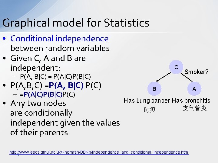
Graphical model for Statistics • Conditional independence between random variables • Given C, A and B are independent: C – P(A, B|C) = P(A|C)P(B|C) • P(A, B, C) =P(A, B|C) P(C) – =P(A|C)P(B|C)P(C) Smoker? B A Has Lung cancer Has bronchitis • Any two nodes 支气管炎肺癌 are conditionally independent given the values of their parents. http: //www. eecs. qmul. ac. uk/~norman/BBNs/Independence_and_conditional_independence. htm 6

Directed and undirected graphical model C • Directed graphical model – P(A, B, C) = P(A|C)P(B|C)P(C) – Any two nodes are conditionally independent given the values of their parents. B A C • Undirected graphical model – P(A, B, C) = P(B, C)P(A, C) – Also called Marcov Random Field (MRF) B A C C B B A 7 D P(A, B, C, D) = P(D|A, B)P(B|C)P(A|C)P(C) A

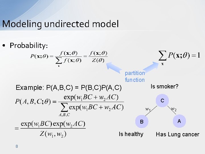
Modeling undirected model • Probability: partition function Is smoker? Example: P(A, B, C) = P(B, C)P(A, C) C w 1 B Is healthy 8 w 2 A Has Lung cancer

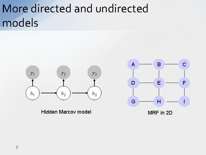
More directed and undirected models y 1 h 1 y 2 h 2 Hidden Marcov model 9 A B C D E F G H I y 3 h 3 MRF in 2 D

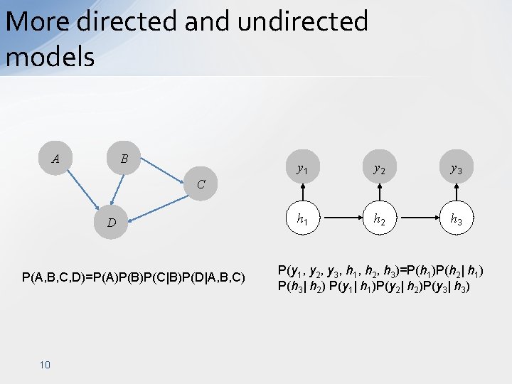
More directed and undirected models A B y 1 y 2 y 3 h 1 h 2 h 3 C D P(A, B, C, D)=P(A)P(B)P(C|B)P(D|A, B, C) 10 P(y 1, y 2, y 3, h 1, h 2, h 3)=P(h 1)P(h 2| h 1) P(h 3| h 2) P(y 1| h 1)P(y 2| h 2)P(y 3| h 3)

More directed and undirected models 11

Extended reading on graphical model • Zoubin Ghahramani ‘s video lecture on graphical models: • http: //videolectures. net/mlss 07_ghahramani_grafm/ 12

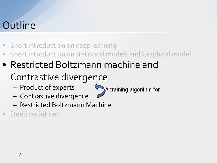
Outline • Short introduction on deep learning • Short introduction on statistical models and Graphical model • Restricted Boltzmann machine and Contrastive divergence – Product of experts A training algorithm for – Contrastive divergence – Restricted Boltzmann Machine • Deep belief net 13

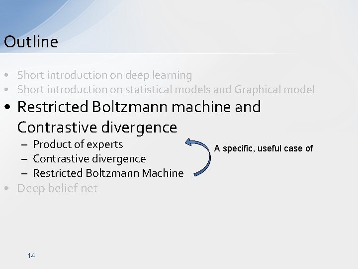
Outline • Short introduction on deep learning • Short introduction on statistical models and Graphical model • Restricted Boltzmann machine and Contrastive divergence – Product of experts – Contrastive divergence – Restricted Boltzmann Machine • Deep belief net 14 A specific, useful case of

Outline • Short introduction on deep learning • Short introduction on statistical models and Graphical model • Restricted Boltzmann machine and Contrastive divergence – Product of experts – Contrastive divergence – Restricted Boltzmann Machine • Deep belief net 15

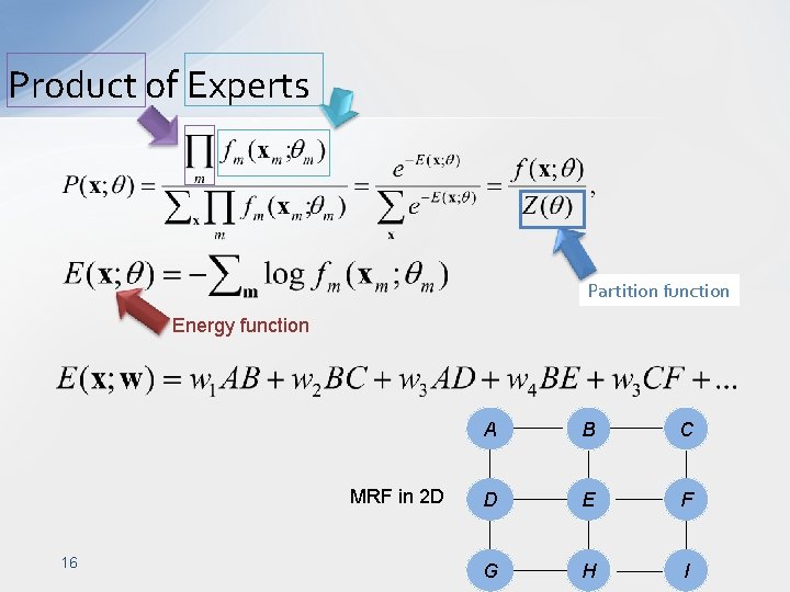
Product of Experts Partition function Energy function MRF in 2 D 16 A B C D E F G H I

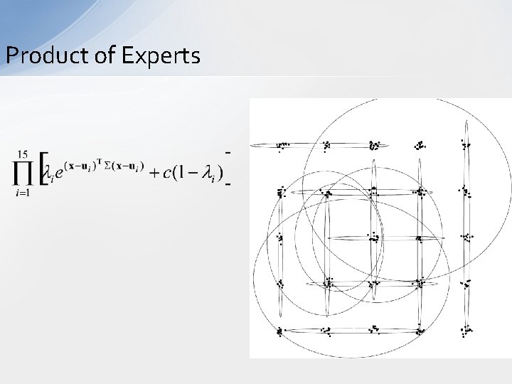
Product of Experts

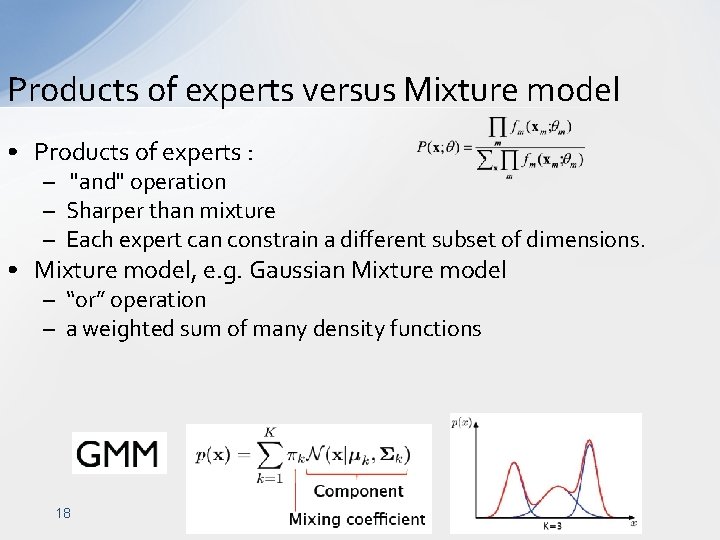
Products of experts versus Mixture model • Products of experts : – "and" operation – Sharper than mixture – Each expert can constrain a different subset of dimensions. • Mixture model, e. g. Gaussian Mixture model – “or” operation – a weighted sum of many density functions 18

Outline • Basic background on statistical learning and Graphical model • Contrastive divergence and Restricted Boltzmann machine – Product of experts – Contrastive divergence – Restricted Boltzmann Machine • Deep belief net 19

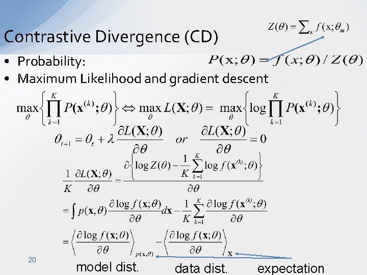
Contrastive Divergence (CD) • Probability: • Maximum Likelihood and gradient descent 20 model dist. data dist. expectation

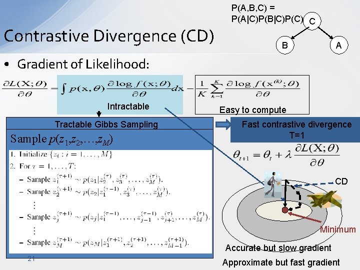
Contrastive Divergence (CD) P(A, B, C) = P(A|C)P(B|C)P(C) C B A • Gradient of Likelihood: Intractable Tractable Gibbs Sampling Sample p(z 1, z 2, …, z. M) Easy to compute Fast contrastive divergence T=1 CD Minimum Accurate but slow gradient 21 Approximate but fast gradient

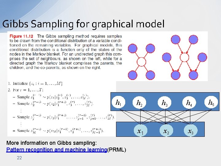
Gibbs Sampling for graphical model h 1 More information on Gibbs sampling: Pattern recognition and machine learning(PRML) 22 h 3 h 4 x 1 x 2 x 3 h 5

Convergence of Contrastive divergence (CD) • The fixed points of ML are not fixed points of CD and vice versa. – CD is a biased learning algorithm. – But the bias is typically very small. – CD can be used for getting close to ML solution and then ML learning can be used for fine-tuning. • It is not clear if CD learning converges (to a stable fixed point). At 2005, proof is not available. • Further theoretical results? Please inform us M. A. Carreira-Perpignan and G. E. Hinton. On Contrastive Divergence Learning. Artificial Intelligence and Statistics, 2005 23

Outline • Basic background on statistical learning and Graphical model • Contrastive divergence and Restricted Boltzmann machine – Product of experts – Contrastive divergence – Restricted Boltzmann Machine • Deep belief net 24

Boltzmann Machine • Undirected graphical model, with hidden nodes. Boltzmann machine: E(x, h)=b' x+c' h+h' Wx+x’Ux+h’Vh 25

Boltzmann machine: E(x, h)=b' x+c' h+h' Wx+x’Ux+h’Vh Restricted Boltzmann Machine (RBM) • Undirected, loopy, layer h 1 partition function • E(x, h)=b' x+c' h+h' Wx h 2 h 3 h 4 x 1 x 2 x 3 h 5 h W x Read the manuscript for details P(xj = 1|h) = σ(bj +W’ • j · h) P(hi = 1|x) = σ(ci +Wi · · x)

Restricted Boltzmann Machine (RBM) • E(x, h)=b' x+c' h+h' Wx • x = [x 1 x 2 …]T, h = [h 1 h 2 …]T • Parameter learning – Maximum Log-Likelihood Geoffrey E. Hinton, “Training Products of Experts by Minimizing Contrastive Divergence. ” Neural Computation 14, 1771– 1800 (2002) 27

CD for RBM • CD for RBM, very fast! CD P(xj = 1|h) = σ(bj +W’ • j · h) 28 P(hi = 1|x) = σ(ci +Wi · x)

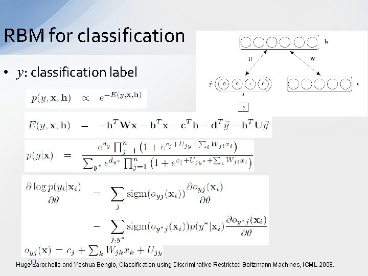
RBM for classification • y: classification label 30 Hugo Larochelle and Yoshua Bengio, Classification using Discriminative Restricted Boltzmann Machines, ICML 2008.

RBM itself has many applications • • • Multiclassification Collaborative filtering Motion capture modeling Information retrieval Modeling natural images Segmentation Y Li, D Tarlow, R Zemel, Exploring compositional high order pattern potentials for structured output learning, CVPR 2013 V. Mnih, H Larochelle, GE Hinton , Conditional Restricted Boltzmann Machines for Structured Output Prediction, Uncertainty in Artificial Intelligence, 2011. Larochelle, H. , & Bengio, Y. (2008). Classification using discriminative restricted boltzmann machines. ICML, 2008. Salakhutdinov, R. , Mnih, A. , & Hinton, G. E. (2007). Restricted Boltzmann machines for collaborative filtering. ICML 2007. Salakhutdinov, R. , & Hinton, G. E. (2009). Replicated softmax: an undirected topic model. , NIPS 2009. Osindero, S. , & Hinton, G. E. (2008). Modeling image patches with a directed hierarchy of markov random field. , NIPS 2008 31

Outline • Basic background on statistical learning and Graphical model • Contrastive divergence and Restricted Boltzmann machine • Deep belief net (DBN) – Why deep leaning? – Learning and inference – Applications 32

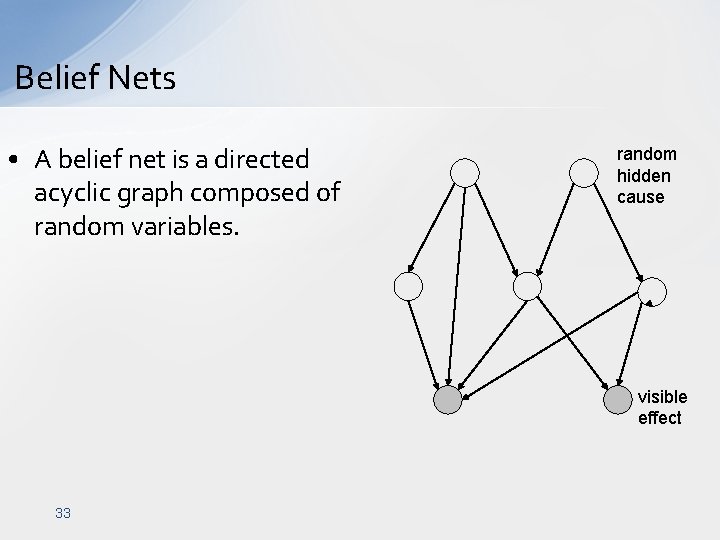
Belief Nets • A belief net is a directed acyclic graph composed of random variables. random hidden cause visible effect 33

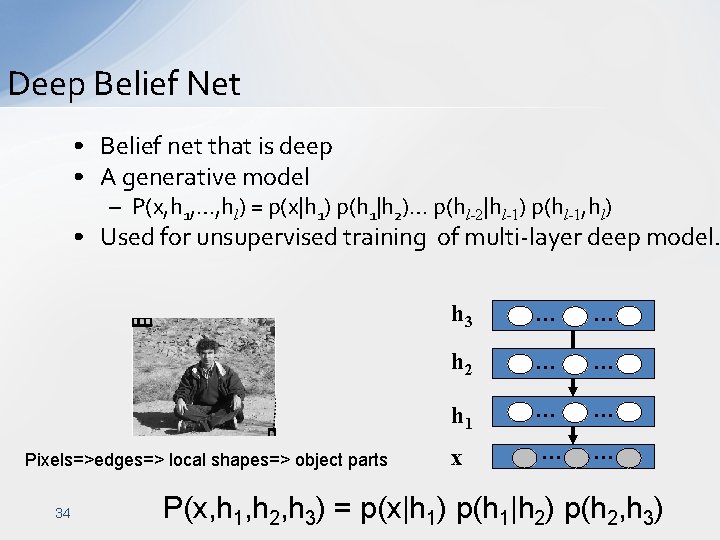
Deep Belief Net • Belief net that is deep • A generative model – P(x, h 1, …, hl) = p(x|h 1) p(h 1|h 2)… p(hl-2|hl-1) p(hl-1, hl) • Used for unsupervised training of multi-layer deep model. Pixels=>edges=> local shapes=> object parts 34 h 3 … … h 2 … … h 1 … … x … … P(x, h 1, h 2, h 3) = p(x|h 1) p(h 1|h 2) p(h 2, h 3)

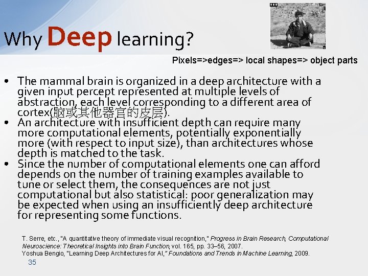
Why Deep learning? Pixels=>edges=> local shapes=> object parts • The mammal brain is organized in a deep architecture with a given input percept represented at multiple levels of abstraction, each level corresponding to a different area of cortex(脑或其他器官的皮层). • An architecture with insufficient depth can require many more computational elements, potentially exponentially more (with respect to input size), than architectures whose depth is matched to the task. • Since the number of computational elements one can afford depends on the number of training examples available to tune or select them, the consequences are not just computational but also statistical: poor generalization may be expected when using an insufficiently deep architecture for representing some functions. T. Serre, etc. , “A quantitative theory of immediate visual recognition, ” Progress in Brain Research, Computational Neuroscience: Theoretical Insights into Brain Function, vol. 165, pp. 33– 56, 2007. Yoshua Bengio, “Learning Deep Architectures for AI, ” Foundations and Trends in Machine Learning, 2009. 35

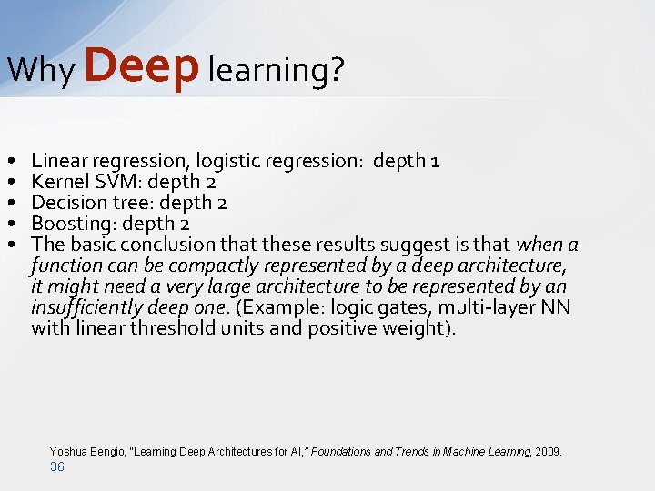
Why Deep learning? • • • Linear regression, logistic regression: depth 1 Kernel SVM: depth 2 Decision tree: depth 2 Boosting: depth 2 The basic conclusion that these results suggest is that when a function can be compactly represented by a deep architecture, it might need a very large architecture to be represented by an insufficiently deep one. (Example: logic gates, multi-layer NN with linear threshold units and positive weight). Yoshua Bengio, “Learning Deep Architectures for AI, ” Foundations and Trends in Machine Learning, 2009. 36

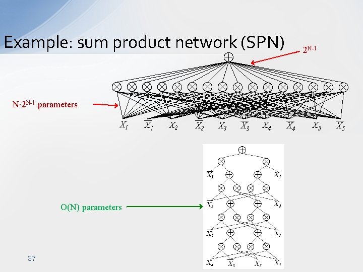
Example: sum product network (SPN) 2 N-1 N 2 N-1 parameters X 1 O(N) parameters 37 X 1 X 2 X 3 X 4 X 5

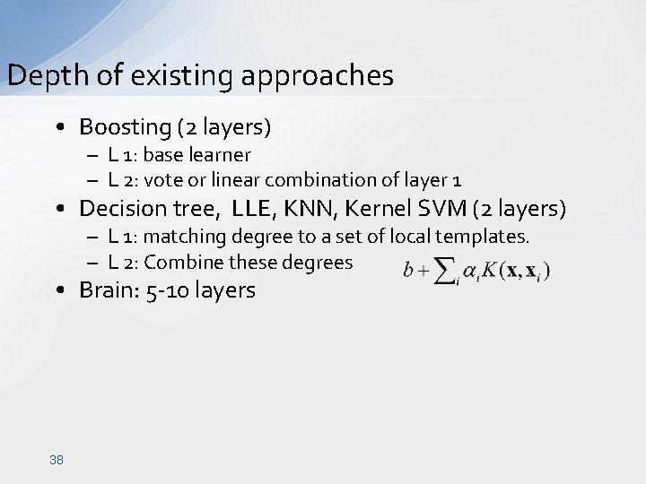
Depth of existing approaches • Boosting (2 layers) – L 1: base learner – L 2: vote or linear combination of layer 1 • Decision tree, LLE, KNN, Kernel SVM (2 layers) – L 1: matching degree to a set of local templates. – L 2: Combine these degrees • Brain: 5 -10 layers 38

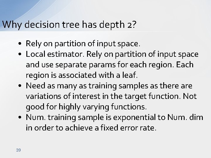
Why decision tree has depth 2? • Rely on partition of input space. • Local estimator. Rely on partition of input space and use separate params for each region. Each region is associated with a leaf. • Need as many as training samples as there are variations of interest in the target function. Not good for highly varying functions. • Num. training sample is exponential to Num. dim in order to achieve a fixed error rate. 39

Outline • Basic background on statistical learning and Graphical model • Contrastive divergence and Restricted Boltzmann machine • Deep belief net (DBN) – Why DBN? – Learning and inference – Applications 40

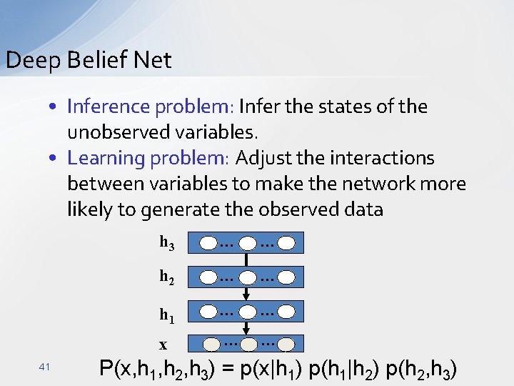
Deep Belief Net • Inference problem: Infer the states of the unobserved variables. • Learning problem: Adjust the interactions between variables to make the network more likely to generate the observed data 41 h 3 … … h 2 … … h 1 … … x … … P(x, h 1, h 2, h 3) = p(x|h 1) p(h 1|h 2) p(h 2, h 3)

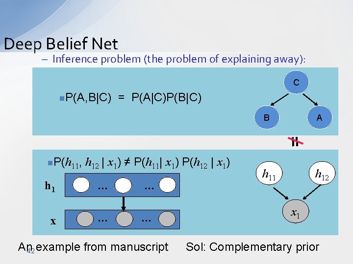
Deep Belief Net – Inference problem (the problem of explaining away): C n. P(A, B|C) = P(A|C)P(B|C) B A = n. P(h 11, h 12 | x 1) ≠ P(h 11| x 1) P(h 12 | x 1) h 1 … … x … … An example from manuscript 42 h 11 h 12 x 1 Sol: Complementary prior

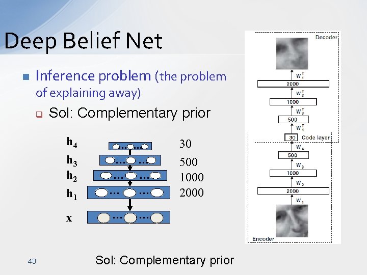
Deep Belief Net n Inference problem (the problem of explaining away) q 43 Sol: Complementary prior h 4 h 3 h 2 h 1 … … … x … … … 30 500 1000 2000 … Sol: Complementary prior

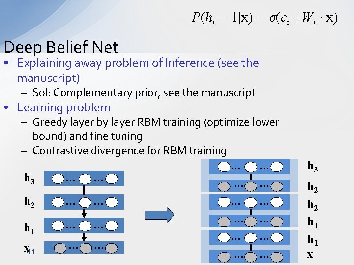
P(hi = 1|x) = σ(ci +Wi · x) Deep Belief Net • Explaining away problem of Inference (see the manuscript) – Sol: Complementary prior, see the manuscript • Learning problem – Greedy layer by layer RBM training (optimize lower bound) and fine tuning – Contrastive divergence for RBM training … … h 3 … … h 2 … … … … h 1 … … x 44 … … h 3 h 2 h 1 x

Code reading • It is much easier to read the Deep. Learning. Toolbox for understanding DBN. 45

46

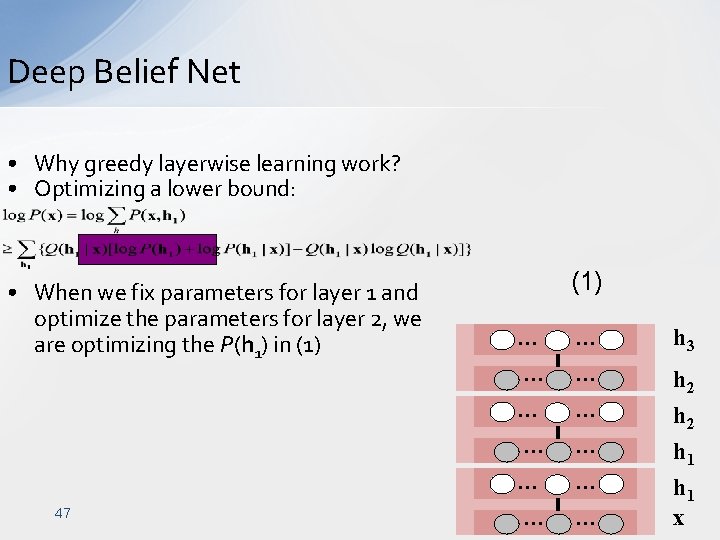
Deep Belief Net • Why greedy layerwise learning work? • Optimizing a lower bound: • When we fix parameters for layer 1 and optimize the parameters for layer 2, we are optimizing the P(h 1) in (1) 47 (1) … … … h 3 h 2 h 1 x

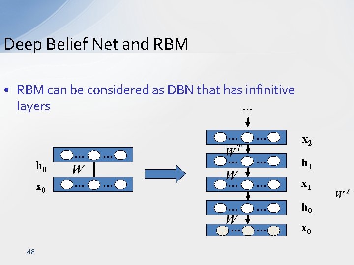
Deep Belief Net and RBM • RBM can be considered as DBN that has infinitive … layers h 0 x 0 48 … … x 2 … … h 1 … … x 1 … … h 0 … … x 0

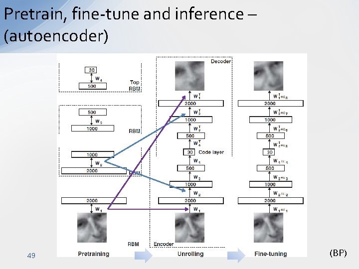
Pretrain, fine-tune and inference – (autoencoder) 49 (BP)

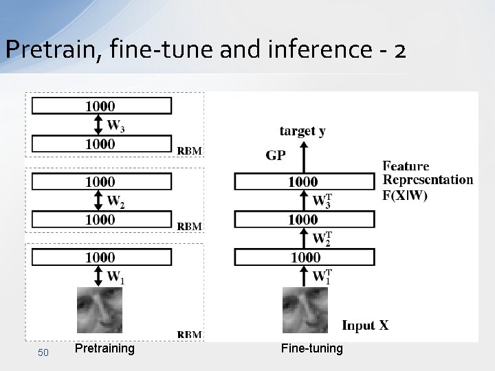
Pretrain, fine-tune and inference - 2 y: identity or rotation degree 50 Pretraining Fine-tuning

How many layers should we use? • There might be no universally right depth – Bengio suggests that several layers is better than one – Results are robust against changes in the size of a layer, but top layer should be big – A parameter. Depends on your task. – With enough narrow layers, we can model any distribution over binary vectors [1] Sutskever, I. and Hinton, G. E. , Deep Narrow Sigmoid Belief Networks are Universal Approximators. Neural Computation, 2007 Copied from http: //videolectures. net/mlss 09 uk_hinton_dbn/ 51

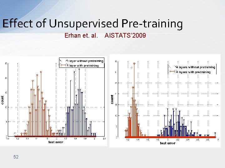
Effect of Unsupervised Pre-training Erhan et. al. AISTATS’ 2009 52

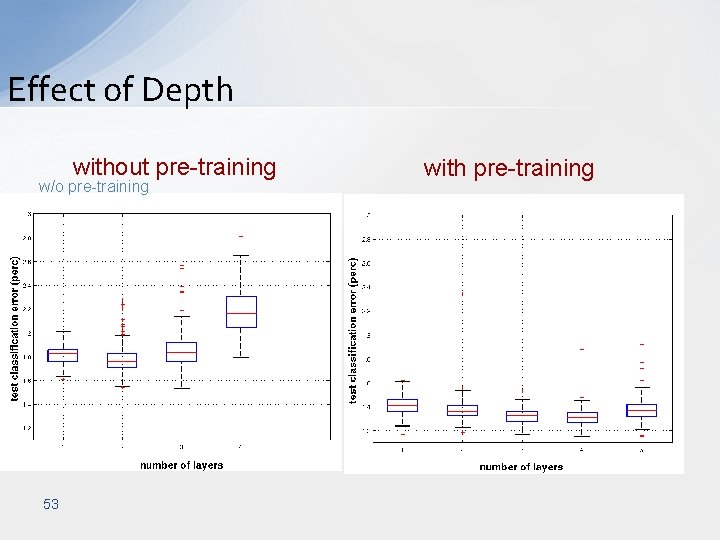
Effect of Depth without pre-training w/o pre-training 53 with pre-training

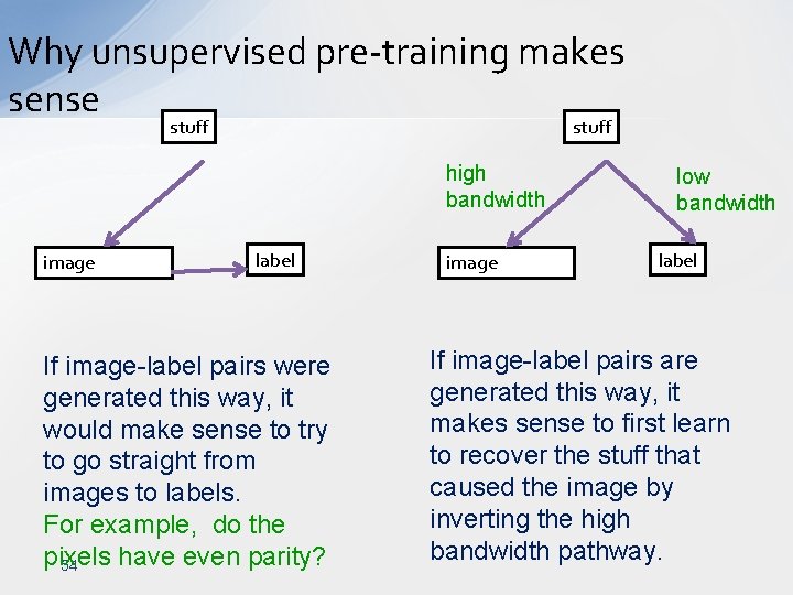
Why unsupervised pre-training makes sense stuff high bandwidth image label If image-label pairs were generated this way, it would make sense to try to go straight from images to labels. For example, do the pixels have even parity? 54 image low bandwidth label If image-label pairs are generated this way, it makes sense to first learn to recover the stuff that caused the image by inverting the high bandwidth pathway.

Beyond layer-wise pretraining • Layer-wise pretraining is efficient but not optimal. • It is possible to train parameters for all layers using a wake-sleep algorithm. – Bottom-up in a layer-wise manner – Top-down and reffiting the earlier models 55

Fine-tuning with a contrastive version of the “wake-sleep” algorithm After learning many layers of features, we can fine-tune the features to improve generation. 1. Do a stochastic bottom-up pass – Adjust the top-down weights to be good at reconstructing the feature activities in the layer below. 2. Do a few iterations of sampling in the top level RBM -- Adjust the weights in the top-level RBM. 3. Do a stochastic top-down pass – Adjust the bottom-up weights to be good at reconstructing the feature activities in the layer above. 56

Include lateral connections • RBM has no connection among layers • This can be generalized. • Lateral connections for the first layer [1]. – Sampling from P(h|x) is still easy. But sampling from p(x|h) is more difficult. • Lateral connections at multiple layers [2]. – Generate more realistic images. – CD is still applicable, with small modification. [1]B. A. Olshausen and D. J. Field, “Sparse coding with an overcomplete basis set: a strategy employed by V 1? , ” Vision Research, vol. 37, pp. 3311– 3325, December 1997. 57 [2]S. Osindero and G. E. Hinton, “Modeling image patches with a directed hierarchy of Markov random field, ” in NIPS, 2007.

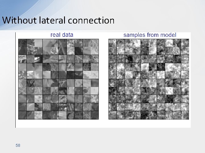
Without lateral connection 58

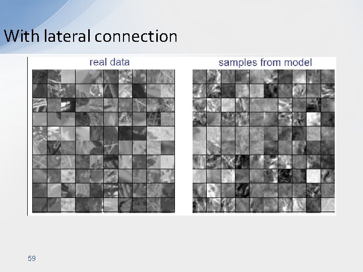
With lateral connection 59

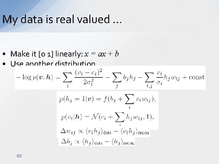
My data is real valued … • Make it [0 1] linearly: x = ax + b • Use another distribution 60

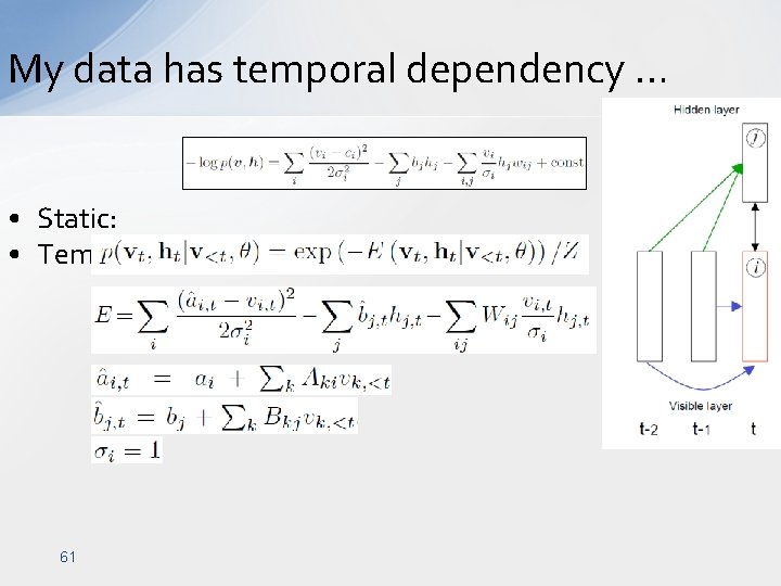
My data has temporal dependency … • Static: • Temporal 61

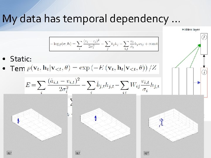
My data has temporal dependency … • Static: • Temporal 62

I consider DBN as… • A statistical model that is used for unsupervised training of fully connected deep model • A directed graphical model that is approximated by fast learning and inference algorithms • A directed graphical model that is fine tuned using mature neural network learning approach -- BP. 63

Outline • Basic background on statistical learning and Graphical model • Contrastive divergence and Restricted Boltzmann machine • Deep belief net (DBN) – Why DBN? – Learning and inference – Applications 64

Applications of deep learning • • • Hand written digits recognition Dimensionality reduction Information retrieval Segmentation Denoising Phone recognition Object detection … Hinton, G. E, Osindero, S. , and Teh, Y. W. (2006). A fast learning algorithm for deep belief nets. Neural Computation Hinton, G. E. and Salakhutdinov, R. R. Reducing the dimensionality of data with neural networks, Science 2006. Welling, M. etc. , Exponential Family Harmoniums with an Application to Information Retrieval, NIPS 2004 A. R. Mohamed, etc. , Deep Belief Networks for phone recognition, NIPS 09 workshop on deep learning for speech recognition. Nair, V. and Hinton, G. E. 3 -D Object recognition with deep belief nets. NIPS 09 ……………. 65

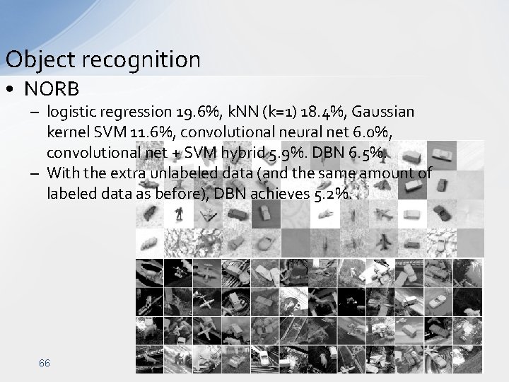
Object recognition • NORB – logistic regression 19. 6%, k. NN (k=1) 18. 4%, Gaussian kernel SVM 11. 6%, convolutional neural net 6. 0%, convolutional net + SVM hybrid 5. 9%. DBN 6. 5%. – With the extra unlabeled data (and the same amount of labeled data as before), DBN achieves 5. 2%. 66

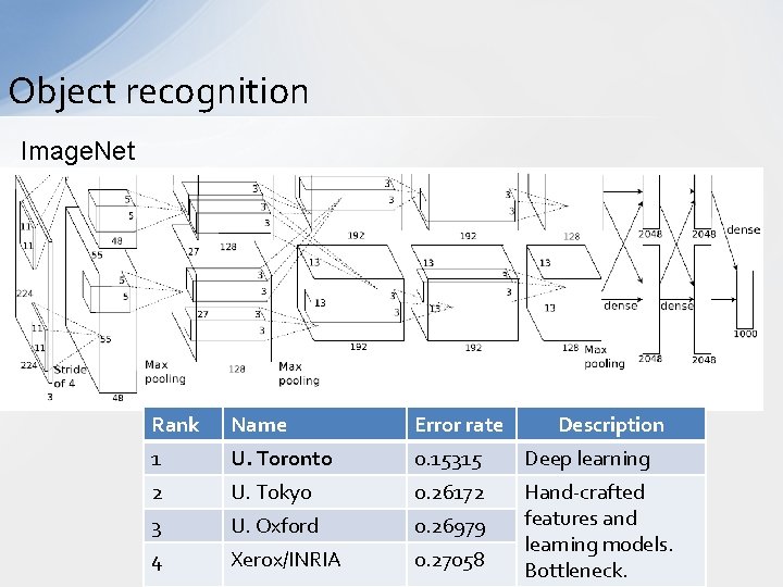
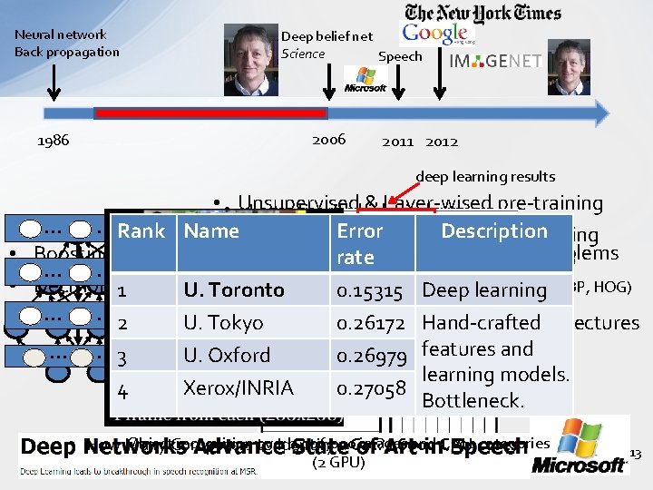
Object recognition Image. Net Rank Name Error rate Description 1 U. Toronto 0. 15315 Deep learning 2 U. Tokyo 0. 26172 3 U. Oxford 0. 26979 4 Xerox/INRIA 0. 27058 Hand-crafted features and 67 learning models. Bottleneck.

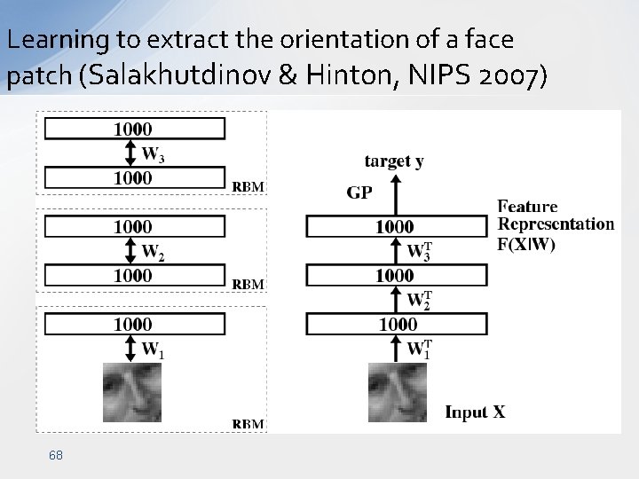
Learning to extract the orientation of a face patch (Salakhutdinov & Hinton, NIPS 2007) 68

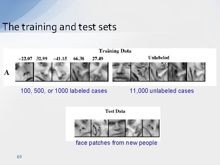
The training and test sets 100, 500, or 1000 labeled cases 11, 000 unlabeled cases face patches from new people 69

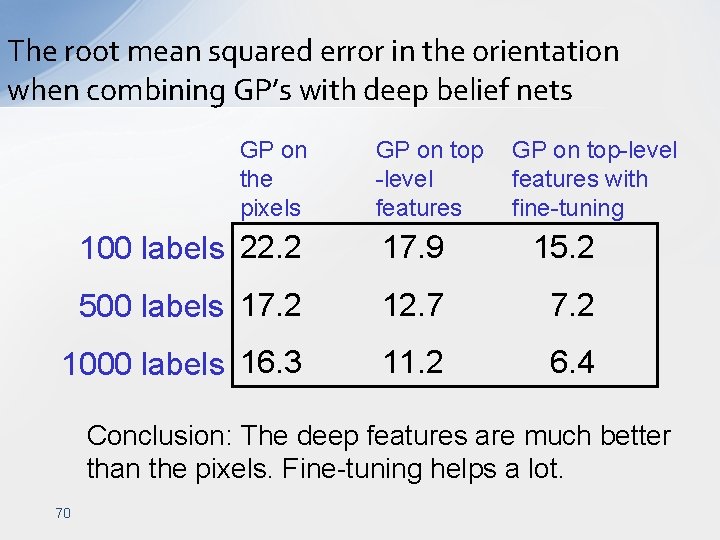
The root mean squared error in the orientation when combining GP’s with deep belief nets GP on the pixels GP on top -level features GP on top-level features with fine-tuning 100 labels 22. 2 17. 9 15. 2 500 labels 17. 2 12. 7 7. 2 1000 labels 16. 3 11. 2 6. 4 Conclusion: The deep features are much better than the pixels. Fine-tuning helps a lot. 70

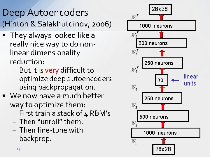
Deep Autoencoders (Hinton & Salakhutdinov, 2006) • They always looked like a really nice way to do nonlinear dimensionality reduction: – But it is very difficult to optimize deep autoencoders using backpropagation. • We now have a much better way to optimize them: – First train a stack of 4 RBM’s – Then “unroll” them. – Then fine-tune with backprop. 71 28 x 28 1000 neurons 500 neurons 250 neurons 30 250 neurons 500 neurons 1000 neurons 28 x 28 linear units

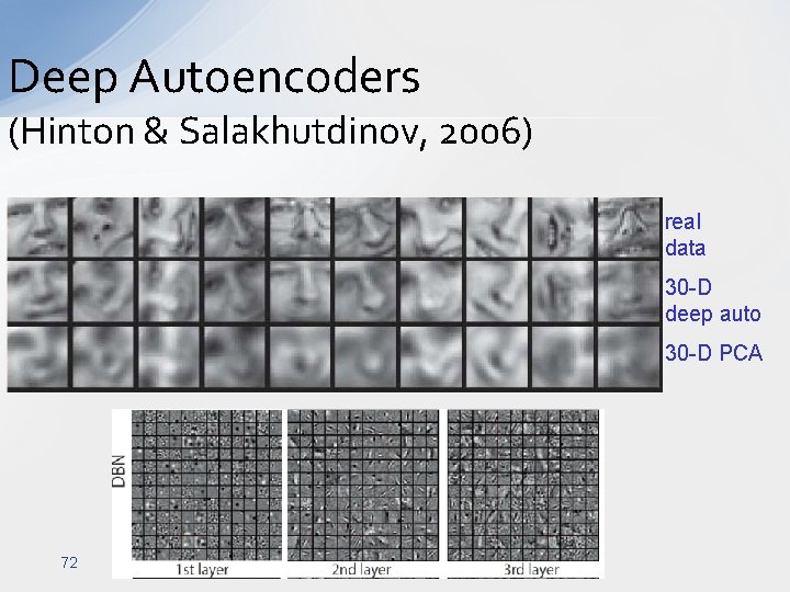
Deep Autoencoders (Hinton & Salakhutdinov, 2006) real data 30 -D deep auto 30 -D PCA 72

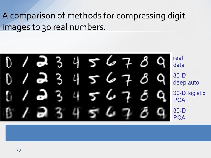
A comparison of methods for compressing digit images to 30 real numbers. real data 30 -D deep auto 30 -D logistic PCA 30 -D PCA 73

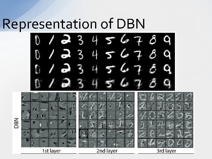
Representation of DBN 74

Our works http: //mmlab. ie. cuhk. edu. hk/project_deep_learning. html 75

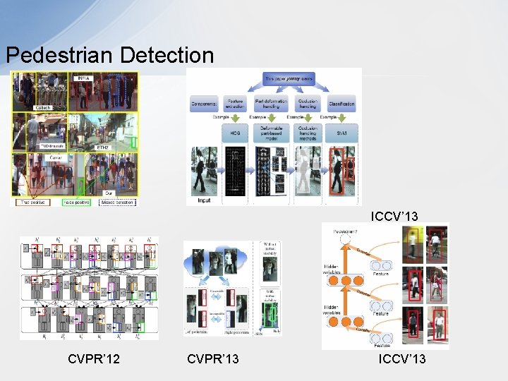
Pedestrian Detection ICCV’ 13 CVPR’ 12 CVPR’ 13 ICCV’ 13

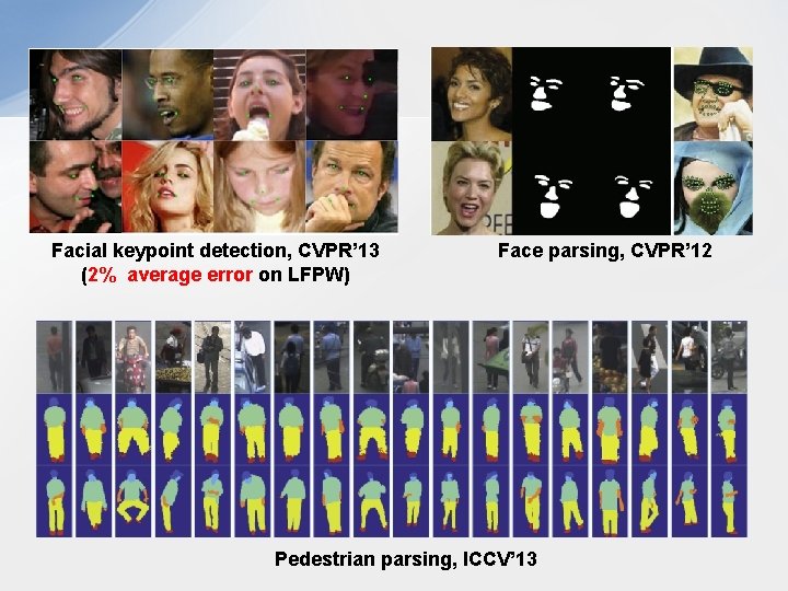
Facial keypoint detection, CVPR’ 13 (2% average error on LFPW) Face parsing, CVPR’ 12 Pedestrian parsing, ICCV’ 13

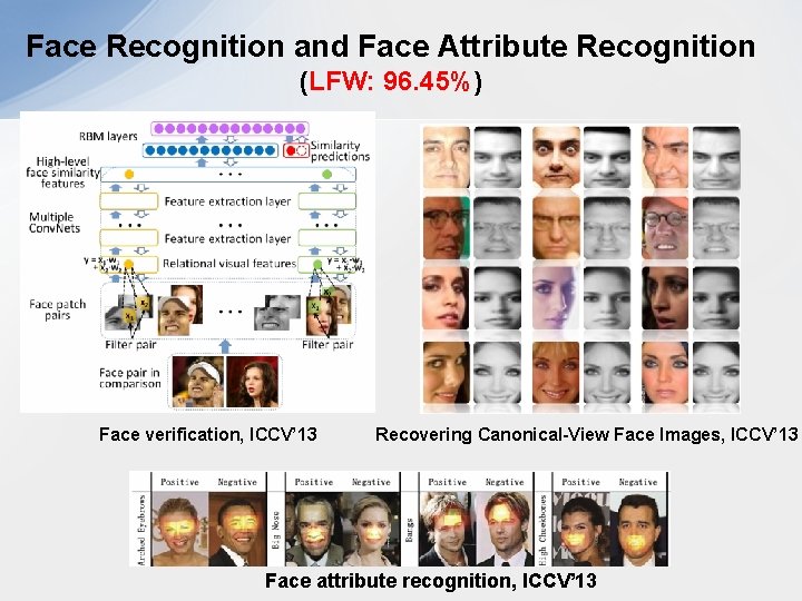
Face Recognition and Face Attribute Recognition (LFW: 96. 45%) Face verification, ICCV’ 13 Recovering Canonical-View Face Images, ICCV’ 13 Face attribute recognition, ICCV’ 13

Summary • Deep belief net (DBN) – is a network with deep layers, which provides strong representation power; – is a generative model; – can be learned by layerwise RBM using Contrastive Divergence; – has many applications and more applications is yet to be found. Generative models explicitly or implicitly model the distribution of inputs and outputs. Discriminative models model the posterior probabilities directly. 79

DBN VS SVM • A very controversial topic • Model – DBN is generative, SVM is discriminative. But fine-tuning of DBN is discriminative • Application – SVM is widely applied. – Researchers are expanding the application area of DBN. • Learning – DBN is non-convex and slow – SVM is convex and fast (in linear case). • Which one is better? – Time will say. – You can contribute Hinton: The superior classification performance of discriminative learning methods holds only for domains in which it is not possible to learn a good generative model. This set of domains is being eroded by Moore’s law. 80

81