Response Times and Their Use in the Cognitive

Response Times and Their Use in the Cognitive Science of Choice Robin Thomas 1, Trish Van Zandt 2, Joe Houpt 3, Mario Fific 4, & Joe Johnson 1 1 Miami University, Oxford, OH 2 The Ohio State University, Columbus, OH 3 Wright State University, Dayton, OH 4 Grand Valley State University, MI

Typical Tasks • Consider a signal detection experiment: one of two stimuli is presented, a standard (or noise) and a comparison (or signal) that differ in intensity on some dimension. The observer must determine which of two occurred on each trial. • A decision maker is given two gambles that differ in value and probability of earnings. Gamble A = 40% chance of winning $10, 60 % chance of losing $5. Gamble B = 60 % chance of winning $6, 40 % chance losing $9. Which does he actually play? How long does it take him to decide?

Typical Tasks • A participant studies a list of items at time t 0. Later, she is presented with another list of items, some old, some new. Her task is to indicate whether each item is old or new. • A learner trains on examples to discover which objects belong in one of two categories (e. g. , friend or foe, poisonous or safe, malignant or benign). New examples are presented to the learner that need to be classified. • Which city is farther south, Paris or New York? How confident are you (on a scale from 0 – 100%)?

In every case, we measure both the choice and the time required to make it.

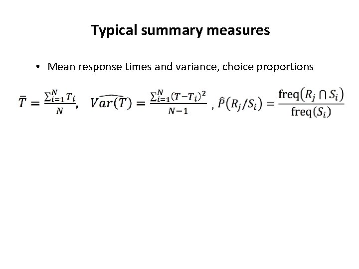
Typical summary measures • Mean response times and variance, choice proportions ,

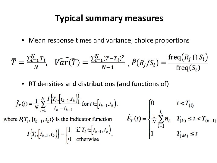
Typical summary measures • Mean response times and variance, choice proportions , • RT densities and distributions (and functions of)

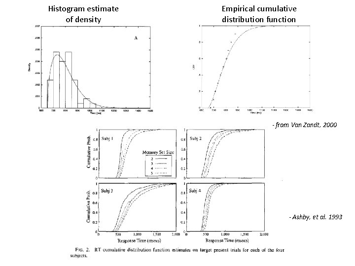
Histogram estimate of density Empirical cumulative distribution function - from Van Zandt, 2000 - Ashby, et al. 1993

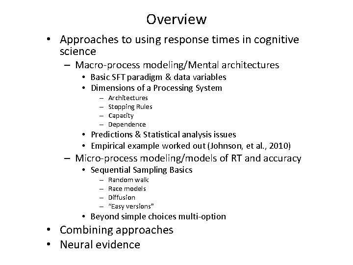
Overview • Approaches to using response times in cognitive science – Macro-process modeling/Mental architectures • Basic SFT paradigm & data variables • Dimensions of a Processing System – – Architectures Stopping Rules Capacity Dependence • Predictions & Statistical analysis issues • Empirical example worked out (Johnson, et al. , 2010) – Micro-process modeling/models of RT and accuracy • Sequential Sampling Basics – – Random walk Race models Diffusion “Easy versions” • Beyond simple choices multi-option • Combining approaches • Neural evidence

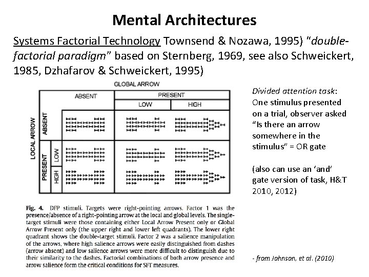
Mental Architectures Systems Factorial Technology Townsend & Nozawa, 1995) “doublefactorial paradigm” based on Sternberg, 1969, see also Schweickert, 1985, Dzhafarov & Schweickert, 1995)

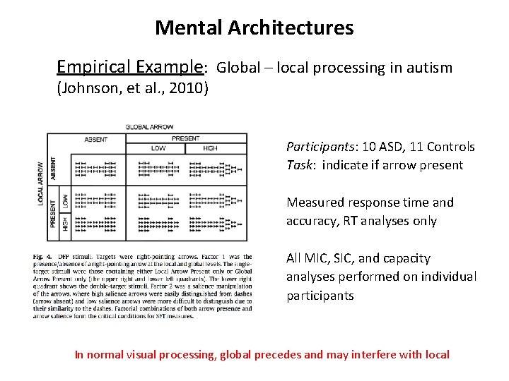
Mental Architectures Systems Factorial Technology Townsend & Nozawa, 1995) “doublefactorial paradigm” based on Sternberg, 1969, see also Schweickert, 1985, Dzhafarov & Schweickert, 1995) Divided attention task: One stimulus presented on a trial, observer asked “Is there an arrow somewhere in the stimulus” = OR gate (also can use an ‘and’ gate version of task, H&T 2010, 2012) - from Johnson, et al. (2010)

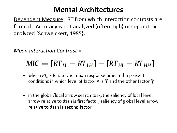
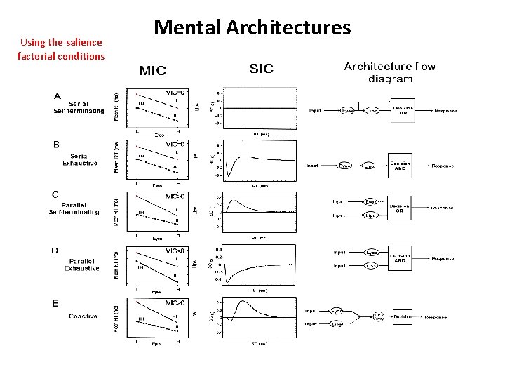
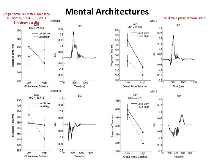
Mental Architectures Dependent Measure: RT from which interaction contrasts are formed. Accuracy is not analyzed (often high) or separately analyzed (Schweickert, 1985). Mean Interaction Contrast = – where Rtij refers to the mean response time in the present conditions in which level of factor A is ‘i’ and the other factor ‘j’ – in the global/local arrow search task, the saliency of local level arrow relative to dash is first factor, saliency of global level arrow relative to dash is second factor

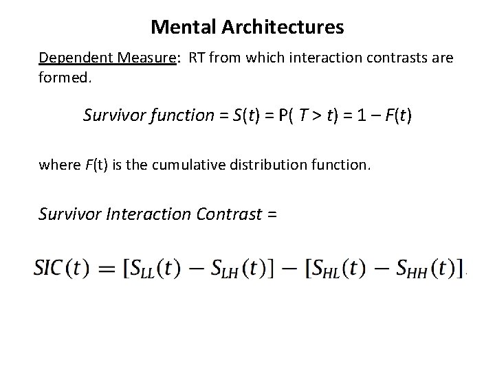
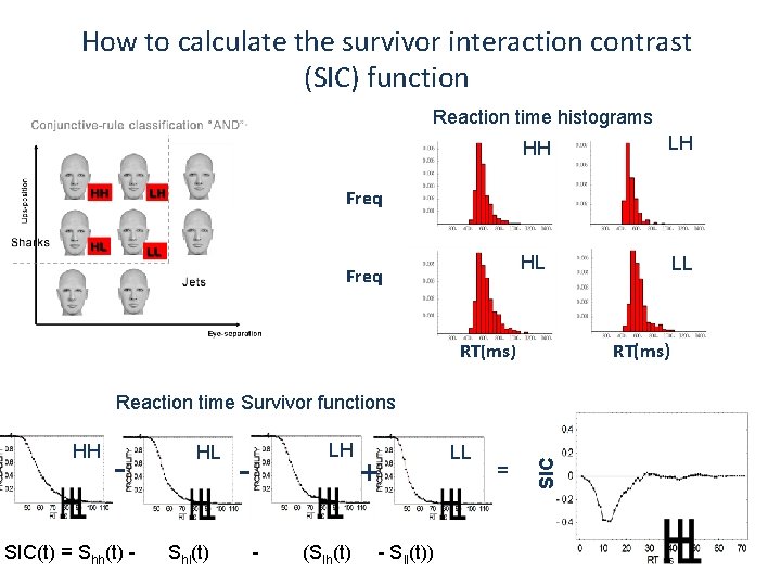
Mental Architectures Dependent Measure: RT from which interaction contrasts are formed. Survivor function = S(t) = P( T > t) = 1 – F(t) where F(t) is the cumulative distribution function. Survivor Interaction Contrast =

How to calculate the survivor interaction contrast (SIC) function Reaction time histograms HH HH LH HL HL LL Freq RT(ms) HH - SIC(t) = Shh(t) - HL Shl(t) LH - (Slh(t) + - Sll(t)) LL = SIC Reaction time Survivor functions

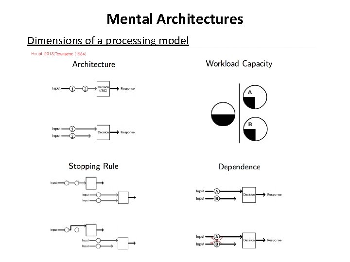
Mental Architectures Dimensions of a processing model

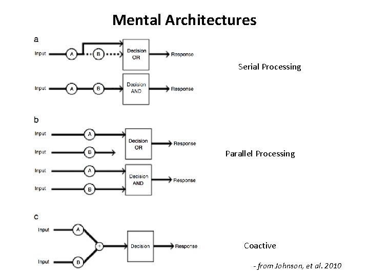
Mental Architectures Serial Processing Parallel Processing Coactive - from Johnson, et al. 2010

Using the salience factorial conditions Mental Architectures

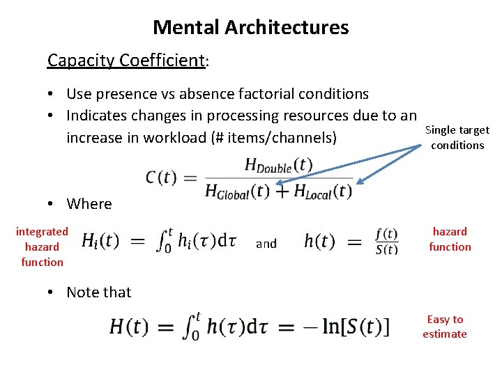
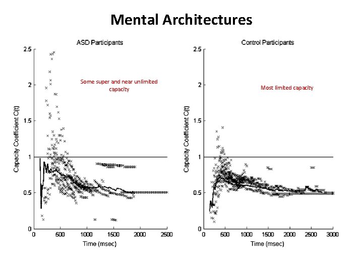
Mental Architectures Capacity Coefficient: • Use presence vs absence factorial conditions • Indicates changes in processing resources due to an increase in workload (# items/channels) Single target conditions • Where integrated hazard function and hazard function • Note that Easy to estimate

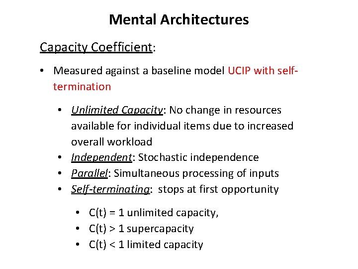
Mental Architectures Capacity Coefficient: • Measured against a baseline model UCIP with selftermination • Unlimited Capacity: No change in resources available for individual items due to increased overall workload • Independent: Stochastic independence • Parallel: Simultaneous processing of inputs • Self-terminating: stops at first opportunity • C(t) = 1 unlimited capacity, • C(t) > 1 supercapacity • C(t) < 1 limited capacity

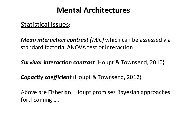
Mental Architectures Statistical Issues: Mean interaction contrast (MIC) which can be assessed via standard factorial ANOVA test of interaction Survivor interaction contrast (Houpt & Townsend, 2010) Capacity coefficient (Houpt & Townsend, 2012) Above are Fisherian. Houpt promises Bayesian approaches forthcoming ….

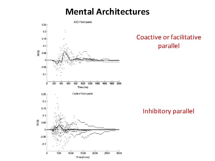
Mental Architectures Empirical Example: Global – local processing in autism (Johnson, et al. , 2010) Participants: 10 ASD, 11 Controls Task: indicate if arrow present Measured response time and accuracy, RT analyses only All MIC, SIC, and capacity analyses performed on individual participants In normal visual processing, global precedes and may interfere with local

Single factor reversal (Townsend & Thomas, 1994) + SIC(t) -> inhibitory parallel Mental Architectures Facilitative parallel exhaustive

Mental Architectures Coactive or facilitative parallel Inhibitory parallel

Mental Architectures Some super and near unlimited capacity Most limited capacity

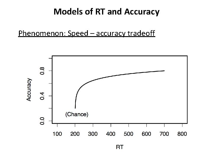
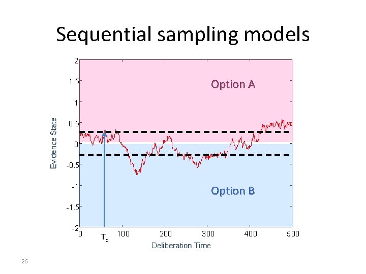
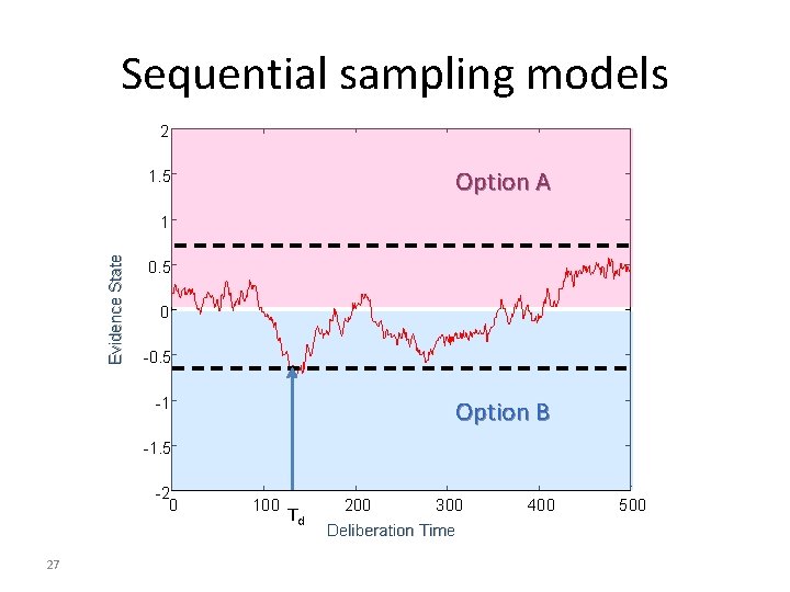
Models of RT and Accuracy SFT uses only RT of correct responses – a weakness of the approach Important information is also included in error responses and the probability of each response especially in classification, memory recognition, decision-making. Predominant approach – sequential sampling • At each moment in time, evidence is accrued according to an underlying stochastic mechanism until enough to determine a response, or time-limit has expired

Models of RT and Accuracy Phenomenon: Speed – accuracy tradeoff

Sequential sampling models 2 Option A 1. 5 Evidence State 1 0. 5 0 -0. 5 -1 Option B -1. 5 -2 0 26 Td 100 200 300 Deliberation Time 400 500

Sequential sampling models 2 Option A 1. 5 Evidence State 1 0. 5 0 -0. 5 -1 Option B -1. 5 -2 0 27 100 Td 200 300 Deliberation Time 400 500

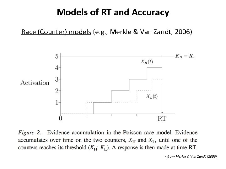
Models of RT and Accuracy Race (Counter) models (e. g. , Merkle & Van Zandt, 2006) - from Merkle & Van Zandt (2006)

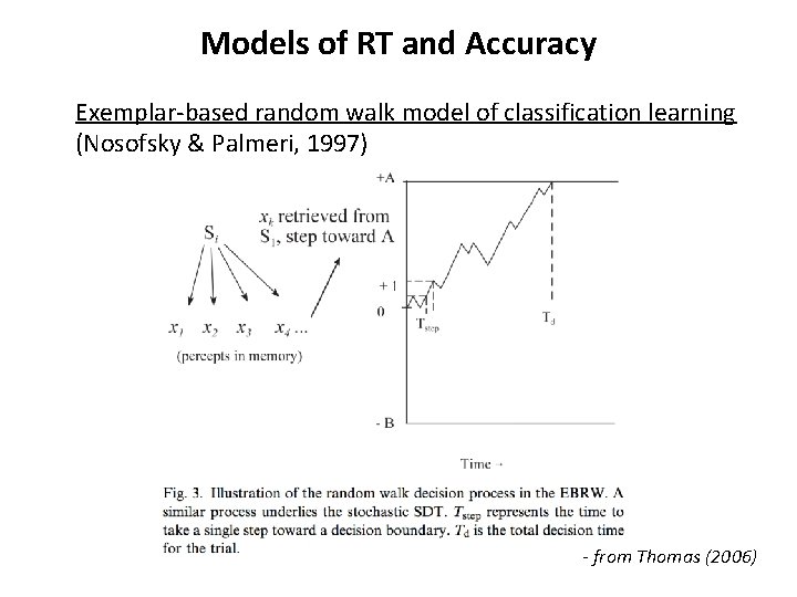
Models of RT and Accuracy Exemplar-based random walk model of classification learning (Nosofsky & Palmeri, 1997) - from Thomas (2006)

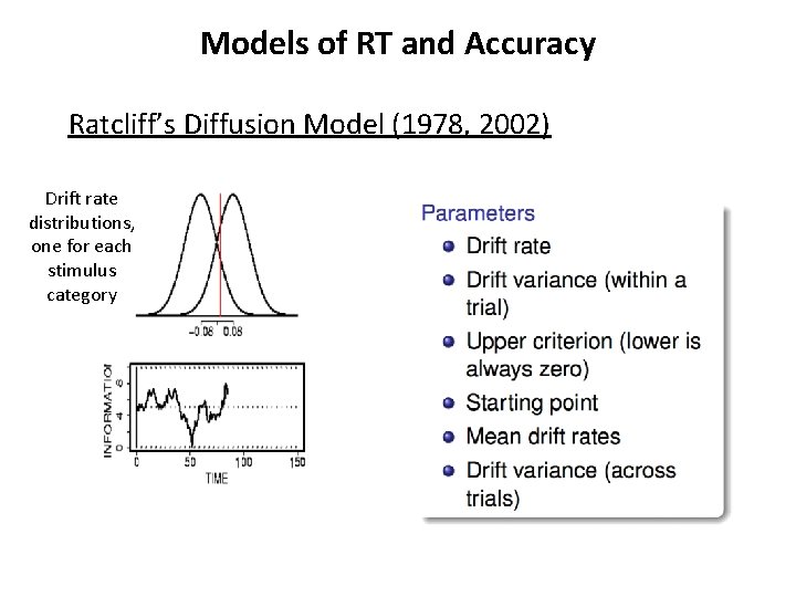
Models of RT and Accuracy Ratcliff’s Diffusion Model (1978, 2002) Drift rate distributions, one for each stimulus category

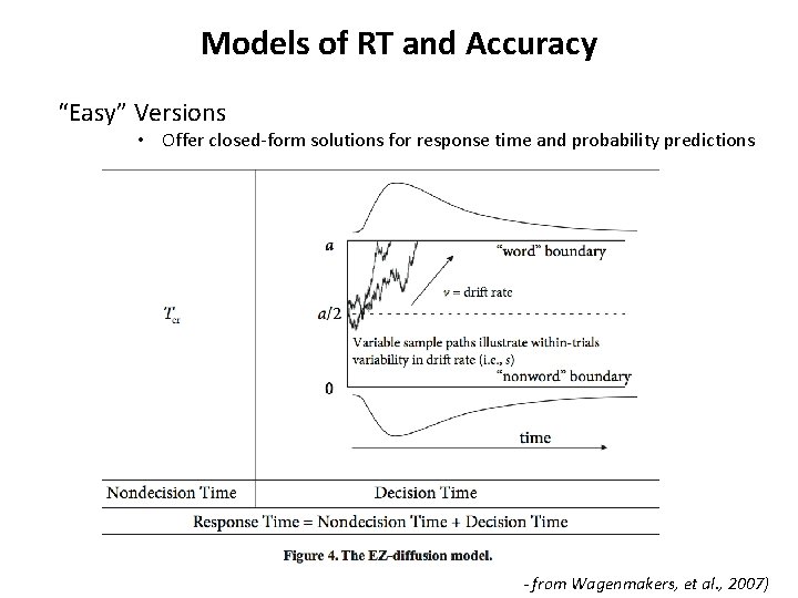
Models of RT and Accuracy “Easy” Versions • Offer closed-form solutions for response time and probability predictions - from Wagenmakers, et al. , 2007)

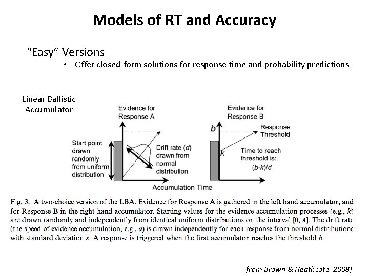
Models of RT and Accuracy “Easy” Versions • Offer closed-form solutions for response time and probability predictions Linear Ballistic Accumulator - from Brown & Heathcote, 2008)

Models of RT and Accuracy Beyond two-choices: Decision Field Theory of Multialternative Decisions (Busemeyer & Townsend, 1993; Johnson & Busemeyer, 2005, 2008) - Attention shifts at each moment to a particular dimension of the decision problem - An evaluation of each choice alternative is based on relative values on the focal dimension - This evaluation is used to update the preference state from the previous moment - Preference updating continues until an alternative surpasses a decision threshold

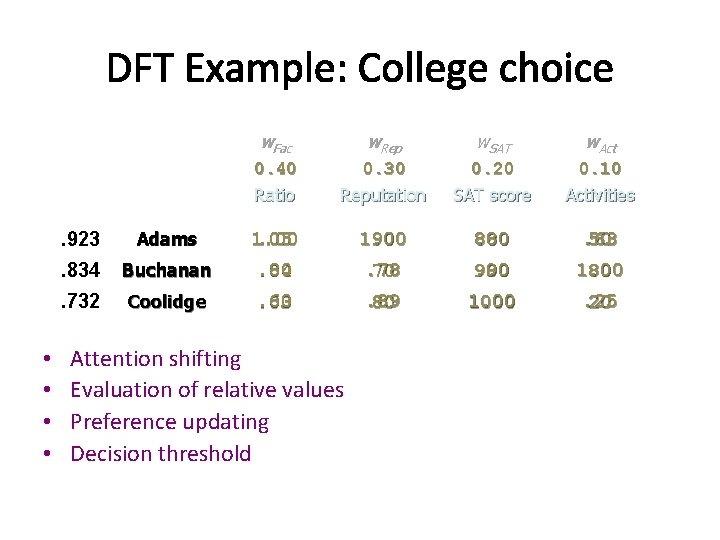
DFT Example: College choice • • w. Fac w. Rep w. SAT w. Act 0. 40 Ratio 0. 30 Reputation 0. 20 SAT score 0. 10 Activities 1. 00 90. 78 70 . 80 800. 90 900 . 63 50 1. 00 80 . 89 80 1. 00 1000 . 25 20 . 923 Adams . 834 Buchanan 1. 00. 05. 80. 04 . 732 Coolidge . 60. 03 Attention shifting Evaluation of relative values Preference updating Decision threshold

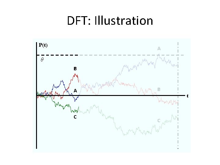
DFT: Illustration P(t) A θ B A C B C t

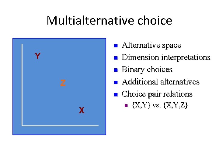
Multialternative choice n Y n n Z n n X Alternative space Dimension interpretations Binary choices Additional alternatives Choice pair relations n {X, Y} vs. {X, Y, Z}

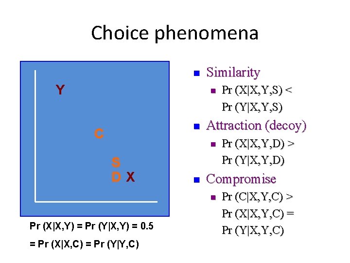
Choice phenomena n Y Similarity n n C Attraction (decoy) n S DX n = Pr (X|X, C) = Pr (Y|Y, C) Pr (X|X, Y, D) > Pr (Y|X, Y, D) Compromise n Pr (X|X, Y) = Pr (Y|X, Y) = 0. 5 Pr (X|X, Y, S) < Pr (Y|X, Y, S) Pr (C|X, Y, C) > Pr (X|X, Y, C) = Pr (Y|X, Y, C)

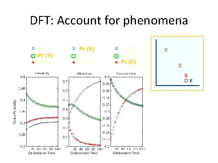
DFT: Account for phenomena x Pr (X) Pr (Y) + Pr (S) x Pr (X) Pr (Y) + Pr (D) x Pr (X) Pr (Y) + Pr (C) Y C S DX

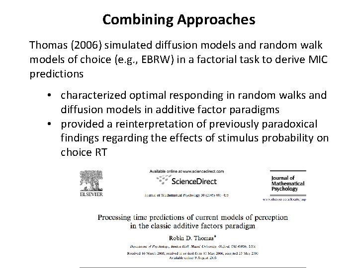
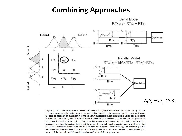
Combining Approaches Thomas (2006) simulated diffusion models and random walk models of choice (e. g. , EBRW) in a factorial task to derive MIC predictions • characterized optimal responding in random walks and diffusion models in additive factor paradigms • provided a reinterpretation of previously paradoxical findings regarding the effects of stimulus probability on choice RT

Combining Approaches

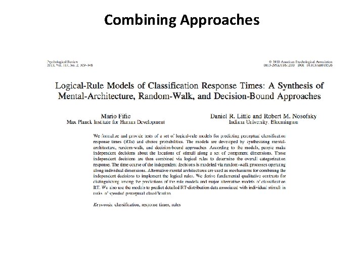
Combining Approaches - Fific, et al. , 2010

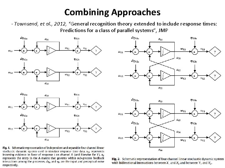
Combining Approaches - Townsend, et al. , 2012, “General recognition theory extended to include response times: Predictions for a class of parallel systems”, JMP

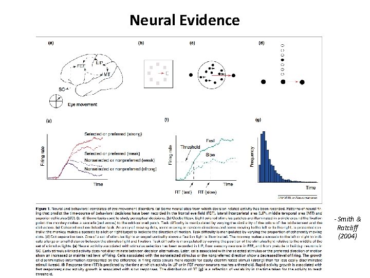
Neural Evidence - Smith & Ratcliff (2004)

Neural Evidence

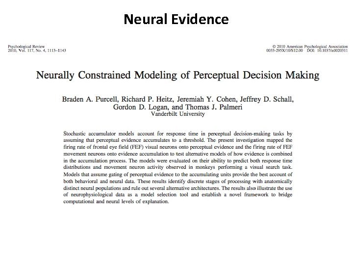
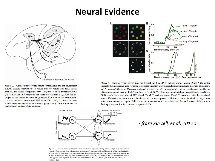
Neural Evidence - from Purcell, et al. 20120

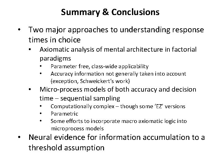
Summary & Conclusions • Two major approaches to understanding response times in choice • Axiomatic analysis of mental architecture in factorial paradigms • • • Parameter free, class-wide applicability Accuracy information not generally taken into account (exception, Schweickert’s work) Micro-process models of both accuracy and decision time – sequential sampling • • • Computationally complex – though some ‘EZ’ versions Parametric Some efforts to incorporate macro axiomatic logic into microprocess models • Neural evidence for information accumulation to a threshold assumption