Resource Signal Prediction and Its Application to Realtime

Resource Signal Prediction and Its Application to Real-time Scheduling Advisors or How to Tame Variability in Distributed Systems Peter A. Dinda Carnegie Mellon University

Outline • Bird’s eye view • • • Highly variable resource availability Real-time scheduling advisor Predicting task running times Characterizing variability with confidence intervals Performance results (feasible, practical, useful) • Prototype system • Host load prediction • Traces, structure, linear models, evaluation • RPS Toolkit • Conclusion 2

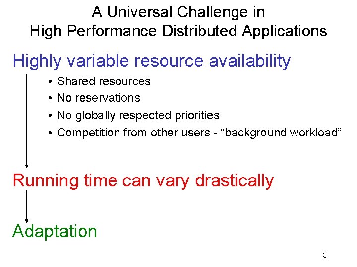
A Universal Challenge in High Performance Distributed Applications Highly variable resource availability • • Shared resources No reservations No globally respected priorities Competition from other users - “background workload” Running time can vary drastically Adaptation 3

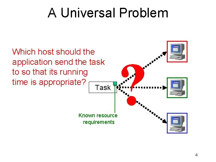
A Universal Problem Which host should the application send the task to so that its running time is appropriate? Task Known resource requirements ? 4

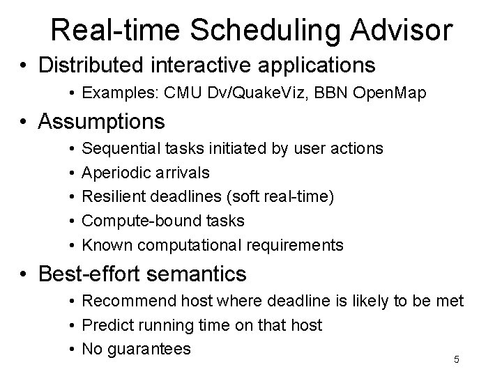
Real-time Scheduling Advisor • Distributed interactive applications • Examples: CMU Dv/Quake. Viz, BBN Open. Map • Assumptions • • • Sequential tasks initiated by user actions Aperiodic arrivals Resilient deadlines (soft real-time) Compute-bound tasks Known computational requirements • Best-effort semantics • Recommend host where deadline is likely to be met • Predict running time on that host • No guarantees 5

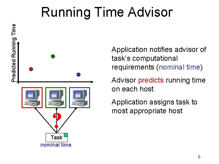
Predicted Running Time Advisor Application notifies advisor of task’s computational requirements (nominal time) Advisor predicts running time on each host ? Application assigns task to most appropriate host Task nominal time 6

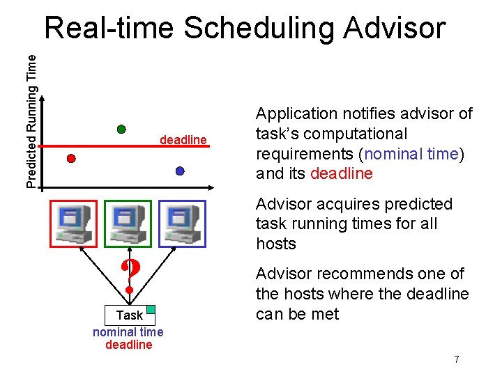
Predicted Running Time Real-time Scheduling Advisor deadline ? Task nominal time deadline Application notifies advisor of task’s computational requirements (nominal time) and its deadline Advisor acquires predicted task running times for all hosts Advisor recommends one of the hosts where the deadline can be met 7

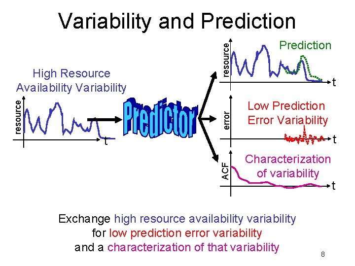
error Prediction t Low Prediction Error Variability t t ACF resource High Resource Availability Variability resource Variability and Prediction Characterization of variability Exchange high resource availability variability for low prediction error variability and a characterization of that variability 8 t

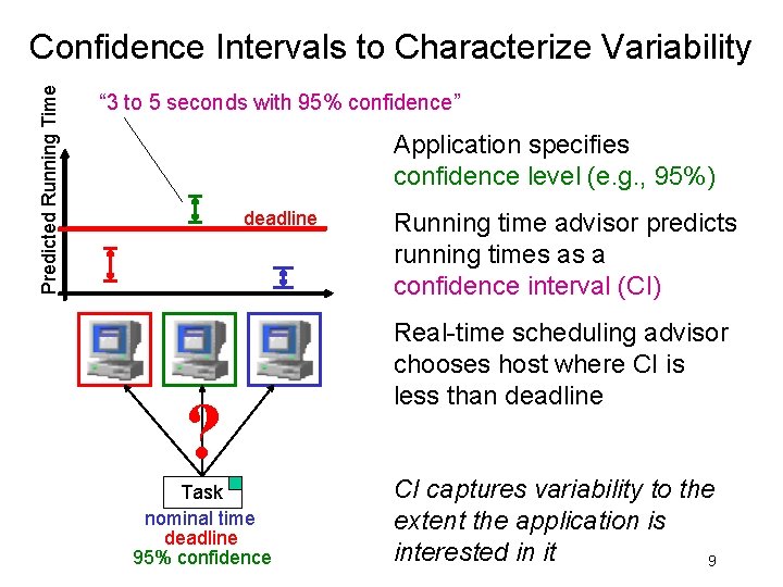
Predicted Running Time Confidence Intervals to Characterize Variability “ 3 to 5 seconds with 95% confidence” Application specifies confidence level (e. g. , 95%) deadline ? Task nominal time deadline 95% confidence Running time advisor predicts running times as a confidence interval (CI) Real-time scheduling advisor chooses host where CI is less than deadline CI captures variability to the extent the application is interested in it 9

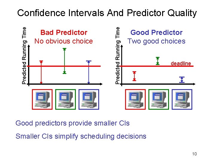
Bad Predictor No obvious choice Predicted Running Time Confidence Intervals And Predictor Quality Good Predictor Two good choices deadline Good predictors provide smaller CIs Smaller CIs simplify scheduling decisions 10

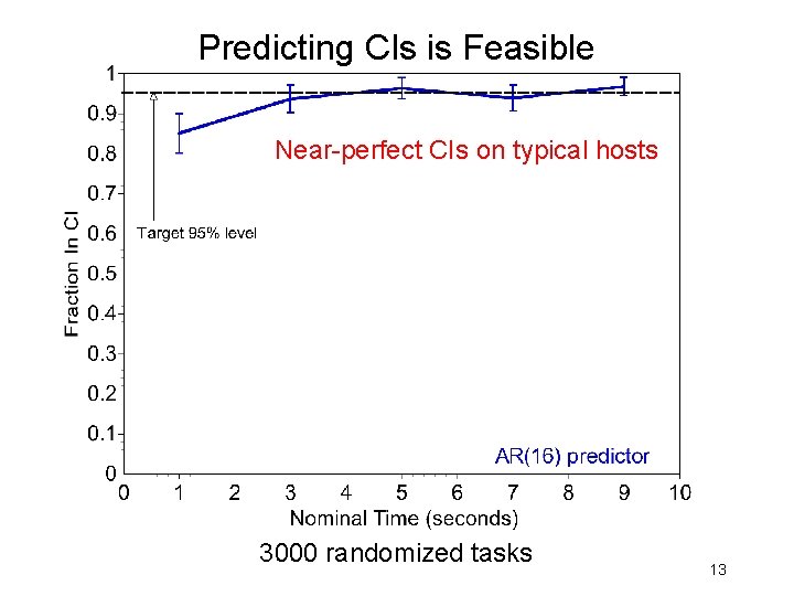
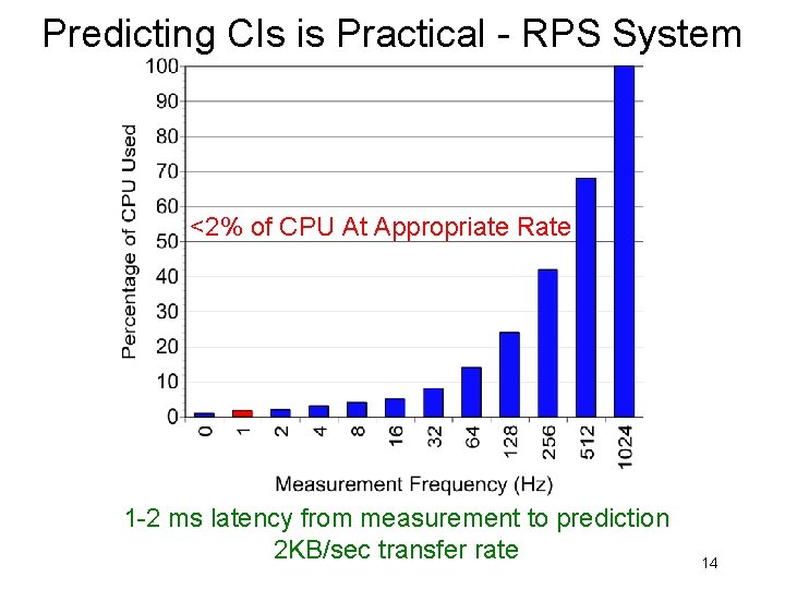
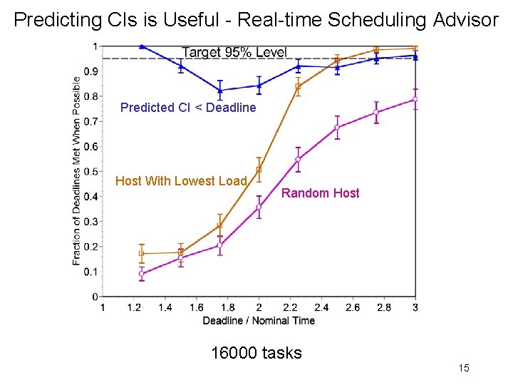
Overview of Research Results • Predicting CIs is feasible • Host load prediction using AR(16) models • Running time estimation using host load predictions • Predicting CIs is practical • RPS Toolkit (inc. in CMU Remos, BBN Qu. O) • Extremely low-overhead online system • Predicting CIs is useful • Performance of real-time scheduling advisor Measured performance of real system Statistically rigorous analysis and evaluation 11

Experimental Setup • Environment – Alphastation 255 s, Digital Unix 4. 0 – Workload: host load trace playback – Prediction system on each host • Tasks – Nominal time ~ U(0. 1, 10) seconds – Interarrival time ~ U(5, 15) seconds • Methodology – Predict CIs / Host recommendations – Run task and measure 12

Predicting CIs is Feasible Near-perfect CIs on typical hosts 3000 randomized tasks 13

Predicting CIs is Practical - RPS System <2% of CPU At Appropriate Rate 1 -2 ms latency from measurement to prediction 2 KB/sec transfer rate 14

Predicting CIs is Useful - Real-time Scheduling Advisor Predicted CI < Deadline Host With Lowest Load Random Host 16000 tasks 15

Outline • Bird’s eye view • • • Highly variable resource availability Real-time scheduling advisor Predicting task running times Characterizing variability with confidence intervals Performance results (feasible, practical, useful) • Prototype system • Host load prediction • Traces, structure, linear models, evaluation • RPS Toolkit • Conclusion 16

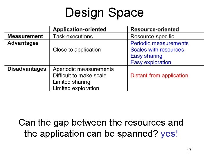
Design Space Can the gap between the resources and the application can be spanned? yes! 17

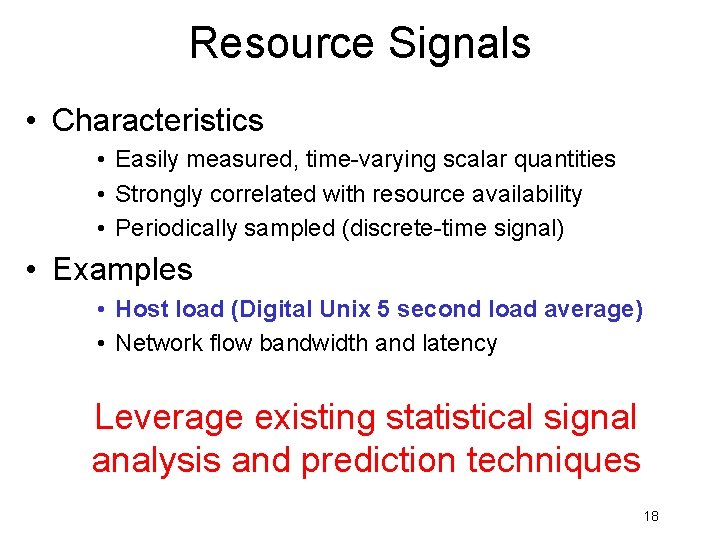
Resource Signals • Characteristics • Easily measured, time-varying scalar quantities • Strongly correlated with resource availability • Periodically sampled (discrete-time signal) • Examples • Host load (Digital Unix 5 second load average) • Network flow bandwidth and latency Leverage existing statistical signal analysis and prediction techniques 18

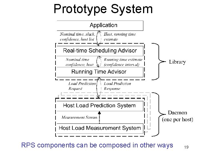
Prototype System RPS components can be composed in other ways 19

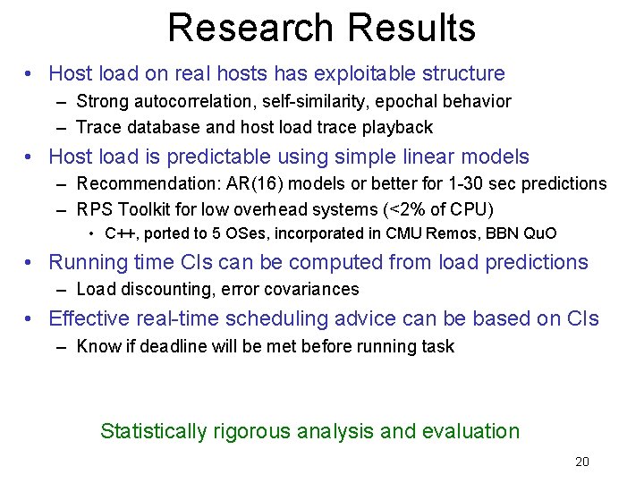
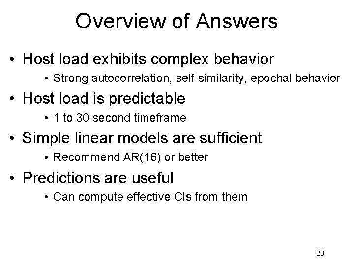
Research Results • Host load on real hosts has exploitable structure – Strong autocorrelation, self-similarity, epochal behavior – Trace database and host load trace playback • Host load is predictable using simple linear models – Recommendation: AR(16) models or better for 1 -30 sec predictions – RPS Toolkit for low overhead systems (<2% of CPU) • C++, ported to 5 OSes, incorporated in CMU Remos, BBN Qu. O • Running time CIs can be computed from load predictions – Load discounting, error covariances • Effective real-time scheduling advice can be based on CIs – Know if deadline will be met before running task Statistically rigorous analysis and evaluation 20

Outline • Bird’s eye view • • • Highly variable resource availability Real-time scheduling advisor Predicting task running times Characterizing variability with confidence intervals Performance results (feasible, practical, useful) • Prototype system • Host load prediction • Traces, structure, linear models, evaluation • RPS Toolkit • Conclusion 21

Questions • • What are the properties of host load? Is host load predictable? What predictive models are appropriate? Are host load predictions useful? 22

Overview of Answers • Host load exhibits complex behavior • Strong autocorrelation, self-similarity, epochal behavior • Host load is predictable • 1 to 30 second timeframe • Simple linear models are sufficient • Recommend AR(16) or better • Predictions are useful • Can compute effective CIs from them 23

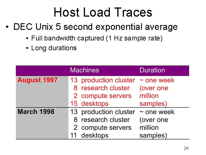
Host Load Traces • DEC Unix 5 second exponential average • Full bandwidth captured (1 Hz sample rate) • Long durations 24

If Host Load Was “Random” (White Noise). . . Time domain Frequency domain Autocorrelation Spectrogram 25

Host Load Has Exploitable Structure Time domain Frequency domain Autocorrelation Spectrogram 26

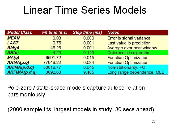
Linear Time Series Models Pole-zero / state-space models capture autocorrelation parsimoniously (2000 sample fits, largest models in study, 30 secs ahead) 27

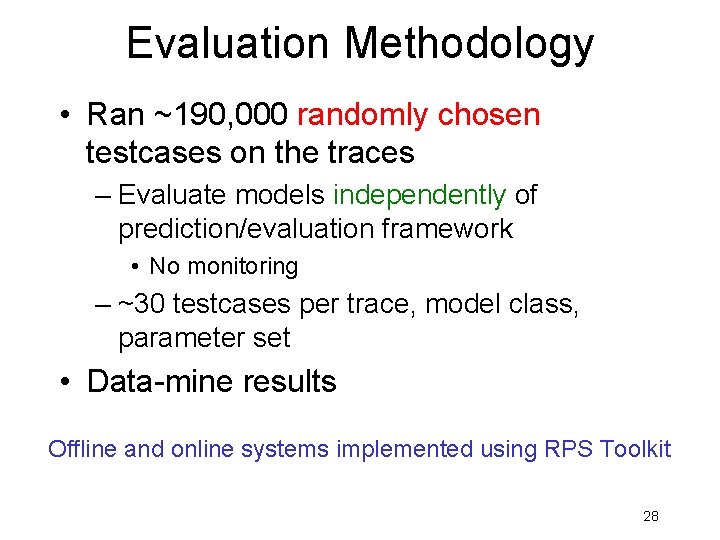
Evaluation Methodology • Ran ~190, 000 randomly chosen testcases on the traces – Evaluate models independently of prediction/evaluation framework • No monitoring – ~30 testcases per trace, model class, parameter set • Data-mine results Offline and online systems implemented using RPS Toolkit 28

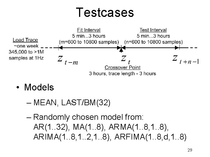
Testcases • Models – MEAN, LAST/BM(32) – Randomly chosen model from: AR(1. . 32), MA(1. . 8), ARMA(1. . 8, 1. . 8), ARIMA(1. . 8, 1. . 2, 1. . 8), ARFIMA(1. . 8, d, 1. . 8) 29

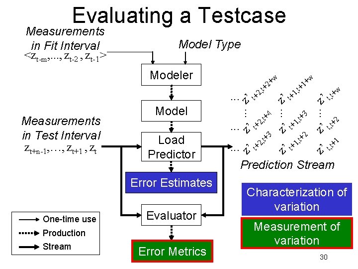
Evaluating a Testcase Model Type Modeler , t . . . Load Predictor Error Estimates One-time use Evaluator Production Stream . . . Measurements in Test Interval zt+n-1, …, zt+1 , zt Model Error Metrics z 4 t+ , 2 t+ ’ z 3 t+ , ’ t+2 +w 1 + , t ’ t+1 . . . ’ t+2 . . . z +w 2 + 3 t+ , 1 z ’ t+1 2 , t+ w ’ t, t+ z. . . Measurements in Fit Interval <zt-m, . . . , zt-2 , zt-1> +2 t , ’t z +1 t , ’t . . . z z z Prediction Stream Characterization of variation Measurement of variation 30

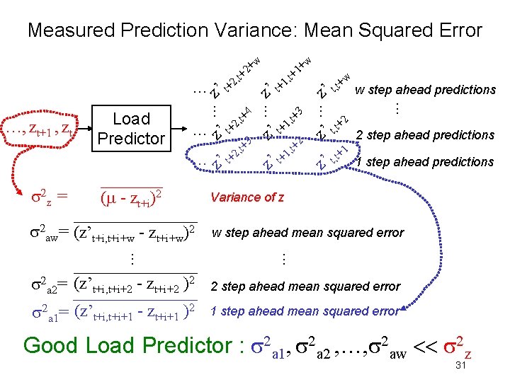
Measured Prediction Variance: Mean Squared Error z 4 t+ 1, 3 . . . z 3 z 2 + t t+ , , 1 t+. . . z’ t+2 ’ z (m - zt+i)2 . . . s 2 aw= (z’t+i, t+i+w - zt+i+w)2 ’ t+ +w t , t z’ w step ahead predictions 2 ’ t, t+ z +1 t , z’ t . . . 1 ’ t+ w 2 step ahead predictions 1 step ahead predictions Variance of z w step ahead mean squared error . . . s 2 z = t+ 2, 1+ + , t . . . …, zt+1 , zt Load Predictor . . . z’ t+2 w . . . 2+ + , t s 2 a 2= (z’t+i, t+i+2 - zt+i+2 )2 2 step ahead mean squared error s 2 a 1= (z’t+i, t+i+1 - zt+i+1 )2 1 step ahead mean squared error Good Load Predictor : s 2 a 1, s 2 a 2 , …, s 2 aw << s 2 z 31

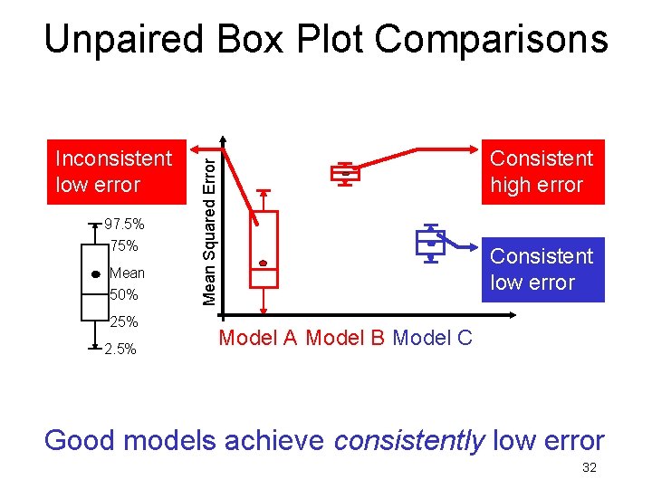
Unpaired Box Plot Comparisons 97. 5% 75% Mean 50% 25% 2. 5% Consistent high error Mean Squared Error Inconsistent low error Consistent low error Model A Model B Model C Good models achieve consistently low error 32

1 second Predictions, All Hosts 97. 5% 75% Mean 50% 25% 2. 5% Predictive models clearly worthwhile 33

30 second Predictions, All Hosts 97. 5% 75% Mean 50% 25% 2. 5% Predictive models clearly beneficial even at long prediction horizons 34

30 Second Predictions, High Load, Dynamic Host 97. 5% 75% Mean 50% 25% 2. 5% Predictive models clearly worthwhile Begin to see differentiation between models 35

RPS Toolkit • Extensible toolkit for implementing resource prediction systems • Easy “buy-in” for users • C++ and sockets (no threads) • Prebuilt prediction components • Libraries (sensors, time series, communication) • Users have bought in • Incorporated in CMU Remos, BBN Qu. O • Used in research by Bruce Lowekamp, Nancy Miller, Le. Monte Green 36

Outline • Bird’s eye view • • • Highly variable resource availability Real-time scheduling advisor Predicting task running times Characterizing variability with confidence intervals Performance results (feasible, practical, useful) • Prototype system • Host load prediction • Traces, structure, linear models, evaluation • RPS Toolkit • Conclusion 37

Related Work • Distributed interactive applications • Quake. Viz/ Dv, Aeschlimann [PDPTA’ 99] • Quality of service • Qu. O, Zinky, Bakken, Schantz [TPOS, April 97] • QRAM, Rajkumar, et al [RTSS’ 97] • Distributed soft real-time systems • Lawrence, Jensen [assorted] • Workload studies for load balancing • Mutka, et al [Perf. Eval ‘ 91] • Harchol-Balter, et al [SIGMETRICS ‘ 96] • Resource signal measurement systems • Remos [HPDC’ 98] • Network Weather Service [HPDC‘ 97, HPDC’ 99] • Host load prediction • Wolski, et al [HPDC’ 99] (NWS) • Samadani, et al [PODC’ 95] • Hailperin [‘ 93] • Application-level scheduling • Berman, et al [HPDC’ 96] • Stochastic Scheduling, Schopf [Supercomputing ‘ 99] 38

Conclusions • Tame variability in distributed systems • Resource signal prediction • Predict running times as confidence intervals – Predicting CIs is feasible • Host load prediction using AR(16) models • Running time estimation using host load predictions – Predicting CIs is practical • RPS Toolkit (inc. in CMU Remos, BBN Qu. O) • Extremely low-overhead online system – Predicting CIs is useful • Performance of real-time scheduling advisor 39

Future Work (Near Term) • New resource signals – Network bandwidth and latency (Remos) • New prediction approaches – Wavelets, nonlinearity • Resource scheduler models – Better Unix scheduler model – Network models • Adaptation advisors • Applications and workloads – Quake. Viz/DV, GIMP, Instrumentation 40

Tools/Venues for Future work • • • Resource signal methodolgy RPS Toolkit Remos Quake. Viz/DV Grid Forum 41

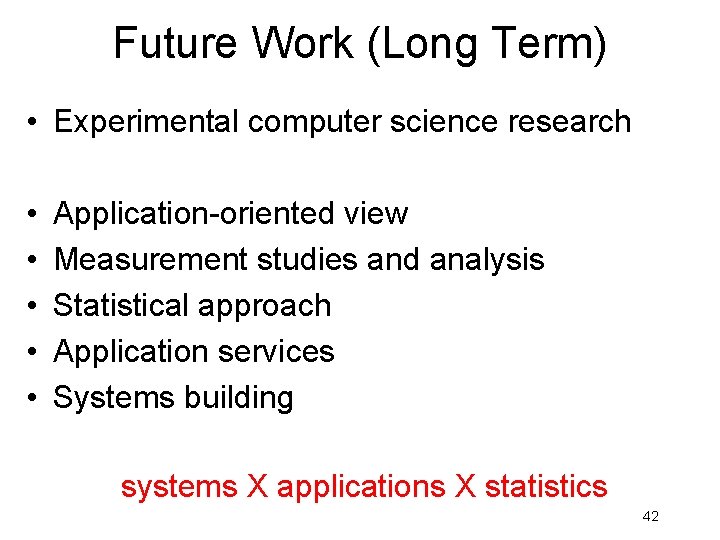
Future Work (Long Term) • Experimental computer science research • • • Application-oriented view Measurement studies and analysis Statistical approach Application services Systems building systems X applications X statistics 42

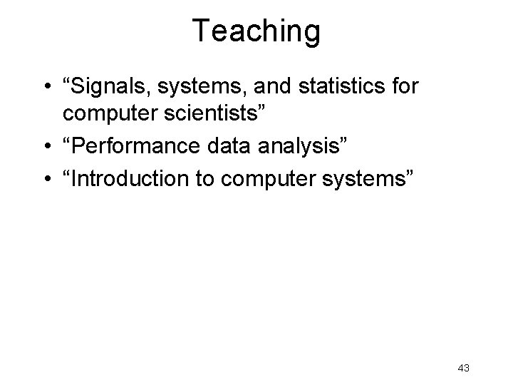
Teaching • “Signals, systems, and statistics for computer scientists” • “Performance data analysis” • “Introduction to computer systems” 43