RESEARCH STATISTICS Normality Sampling Hypothesis Testing and sample

RESEARCH STATISTICS Normality, Sampling & Hypothesis Testing and sample size estimation Jobayer Hossain, Ph. D Larry Holmes, Jr, Ph. D October 23, 2008

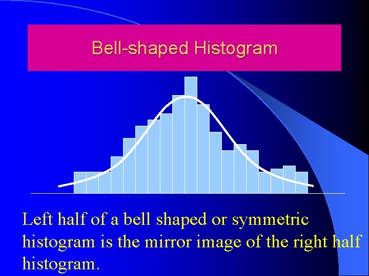
Bell-shaped Histogram Left half of a bell shaped or symmetric histogram is the mirror image of the right half histogram.

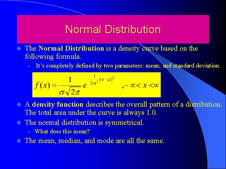
Normal Distribution l The Normal Distribution is a density curve based on the following formula. – It’s completely defined by two parameters: mean; and standard deviation. A density function describes the overall pattern of a distribution. The total area under the curve is always 1. 0. l The normal distribution is symmetrical. l – What does this mean? l The mean, median and mode are all the same.

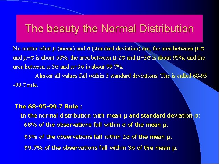
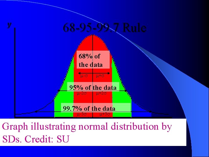
The beauty the Normal Distribution No matter what (mean) and (standard deviation) are, the area between - and + is about 68%; the area between -2 and +2 is about 95%; and the area between -3 and +3 is about 99. 7%. Almost all values fall within 3 standard deviations. The is called 68 -95 -99. 7 rule. The 68 -95 -99. 7 Rule : In the normal distribution with mean µ and standard deviation σ: 68% of the observations fall within σ of the mean µ. 95% of the observations fall within 2σ of the mean µ. 99. 7% of the observations fall within 3σ of the mean µ.

68 -95 -99. 7 Rule 68% of the data - + 95% of the data -2 +2 99. 7% of the data -3 +3 Graph illustrating normal distribution by SDs. Credit: SU

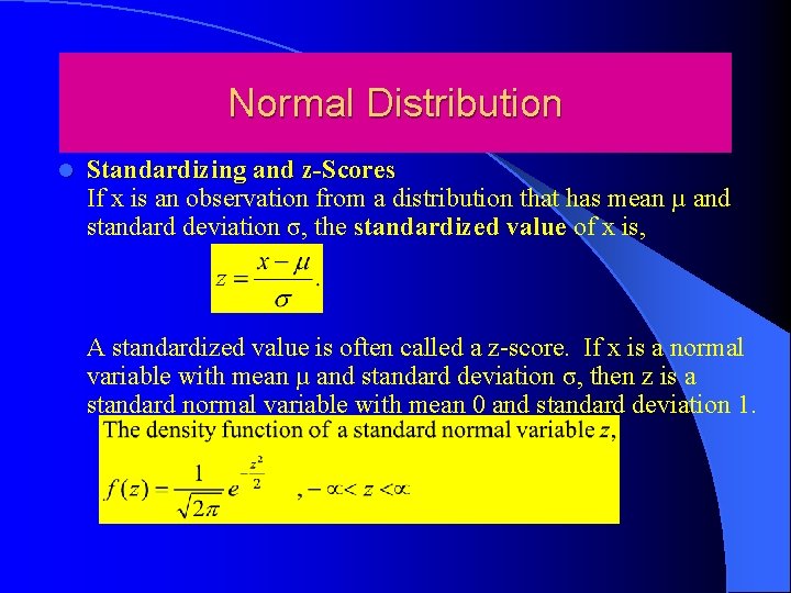
Normal Distribution l Standardizing and z-Scores If x is an observation from a distribution that has mean µ and standard deviation σ, the standardized value of x is, A standardized value is often called a z-score. If x is a normal variable with mean µ and standard deviation σ, then z is a standard normal variable with mean 0 and standard deviation 1.

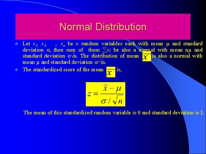
Normal Distribution Let x 1, x 2, …. , xn be n random variables each with mean µ and standard deviation σ, then sum of them ∑xi be also a normal with mean nµ and standard deviation σ√n. The distribution of mean is also a normal with mean µ and standard deviation σ/√n. l The standardized score of the mean is, l The mean of this standardized random variable is 0 and standard deviation is 1.

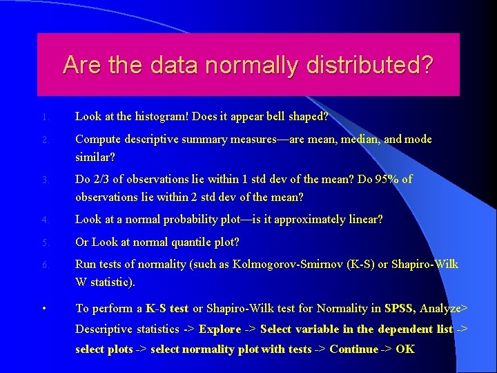
Are the data normally distributed? 1. Look at the histogram! Does it appear bell shaped? 2. Compute descriptive summary measures—are mean, median, and mode similar? 3. Do 2/3 of observations lie within 1 std dev of the mean? Do 95% of observations lie within 2 std dev of the mean? 4. Look at a normal probability plot—is it approximately linear? 5. Or Look at normal quantile plot? 6. Run tests of normality (such as Kolmogorov-Smirnov (K-S) or Shapiro-Wilk W statistic). • To perform a K-S test or Shapiro-Wilk test for Normality in SPSS, Analyze> Descriptive statistics -> Explore -> Select variable in the dependent list -> select plots -> select normality plot with tests -> Continue -> OK

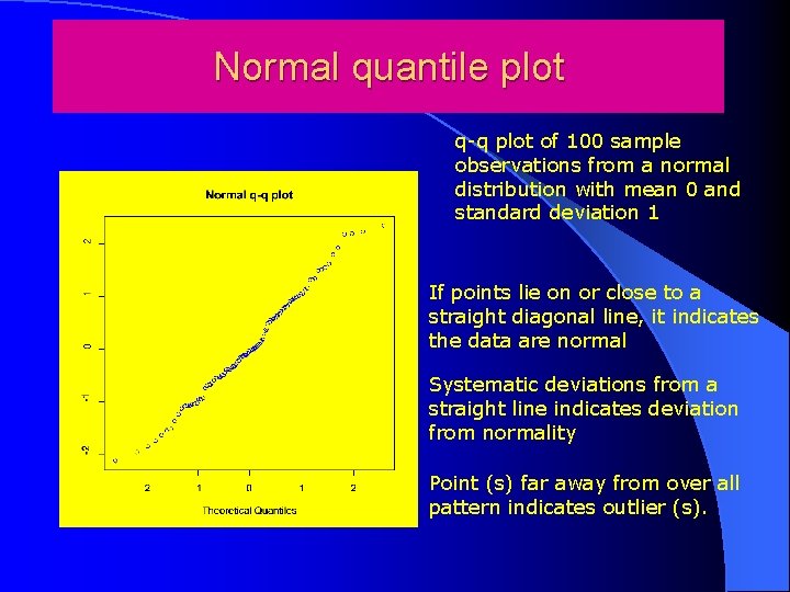
Normal quantile plot q-q plot of 100 sample observations from a normal distribution with mean 0 and standard deviation 1 If points lie on or close to a straight diagonal line, it indicates the data are normal Systematic deviations from a straight line indicates deviation from normality Point (s) far away from over all pattern indicates outlier (s).

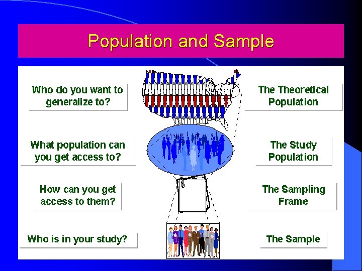
Population and Sample

Population and sample l Population: The entire collection of individuals, objects or measurements that we want information about. l Sample: A subset (part) of the population that we select to examine in order to gather information. – Primary objective is to create a sample so that the distribution of the sample is similar to the distribution of the population. That is to create a subset of population whose center, spread and shape are as close as that of population. – Methods of sampling: Random sampling, stratified sampling, systematic sampling, cluster sampling, multistage sampling, area sampling, qoata sampling etc.

Population and Sample l Random Sample: A simple random sample of size n from a population is a subset of n elements from that population where the subset is chosen in such a way that every possible unit of population has the same chance of being selected. l Example: Consider a population of 5 numbers (1, 2, 3, 4, 5). How many random samples (without replacement) of size 2 can we draw from this population ? (1, 2), (1, 3), (1, 4), (1, 5), (2, 3), (2, 4), (2, 5), (3, 4), (3, 5), (4, 5)

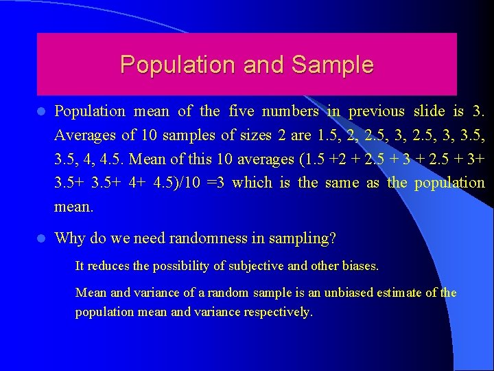
Population and Sample l Population mean of the five numbers in previous slide is 3. Averages of 10 samples of sizes 2 are 1. 5, 2, 2. 5, 3, 3. 5, 4, 4. 5. Mean of this 10 averages (1. 5 +2 + 2. 5 + 3+ 3. 5+ 4+ 4. 5)/10 =3 which is the same as the population mean. l Why do we need randomness in sampling? It reduces the possibility of subjective and other biases. Mean and variance of a random sample is an unbiased estimate of the population mean and variance respectively.

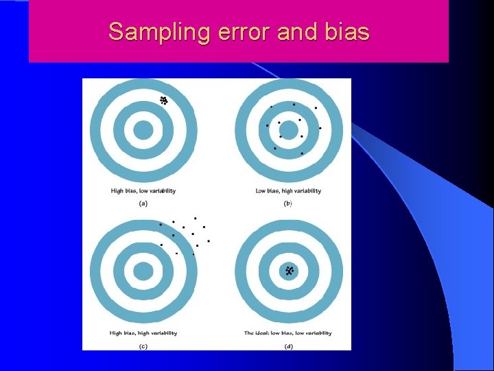
Sampling error and bias

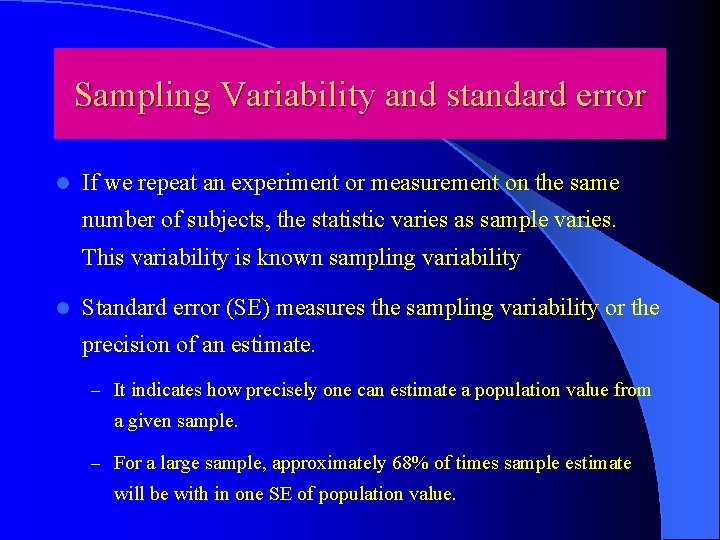
Sampling Variability and standard error l If we repeat an experiment or measurement on the same number of subjects, the statistic varies as sample varies. This variability is known sampling variability l Standard error (SE) measures the sampling variability or the precision of an estimate. – It indicates how precisely one can estimate a population value from a given sample. – For a large sample, approximately 68% of times sample estimate will be with in one SE of population value.

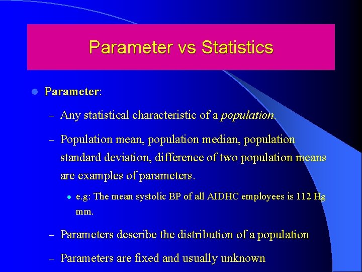
Parameter vs Statistics l Parameter: – Any statistical characteristic of a population. – Population mean, population median, population standard deviation, difference of two population means are examples of parameters. l e. g: The mean systolic BP of all AIDHC employees is 112 Hg mm. – Parameters describe the distribution of a population – Parameters are fixed and usually unknown

Parameter vs Statistic l Statistic: Any statistical characteristic of a sample. – Sample mean, sample median, sample standard deviation, sample proportion, odds ratio, sample correlation coefficient are some examples of statistics. – Mean systolic BP of a sample of 50 AIDHC emplyees or the difference of means systolic BP for a sample of 25 women and 25 men at AIDHC. – Statistic describes the distribution of population – Value of a statistic is known and is varies for different samples – STATISTIC are used for making inference on parameter

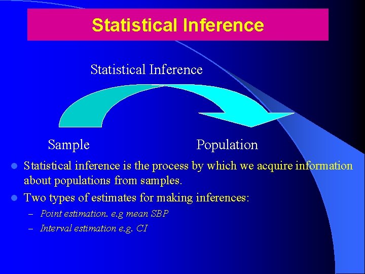
Statistical Inference Sample Population Statistical inference is the process by which we acquire information about populations from samples. l Two types of estimates for making inferences: l – Point estimation. e. g mean SBP – Interval estimation e. g. CI

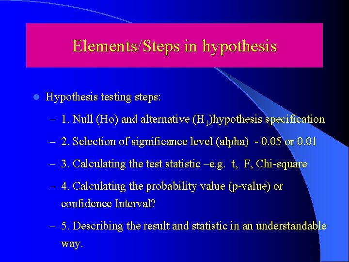
Elements/Steps in hypothesis l Hypothesis testing steps: – 1. Null (Ho) and alternative (H 1)hypothesis specification – 2. Selection of significance level (alpha) - 0. 05 or 0. 01 – 3. Calculating the test statistic –e. g. t, F, Chi-square – 4. Calculating the probability value (p-value) or confidence Interval? – 5. Describing the result and statistic in an understandable way.

What is a Hypothesis? l A hypothesis is an assumption about the population parameter. – A parameter is a characteristic of the population, like its mean or variance. – The parameter (mean) must be identified before analysis. We assume the mean SBP of men at AIDH is 135 Hg mm

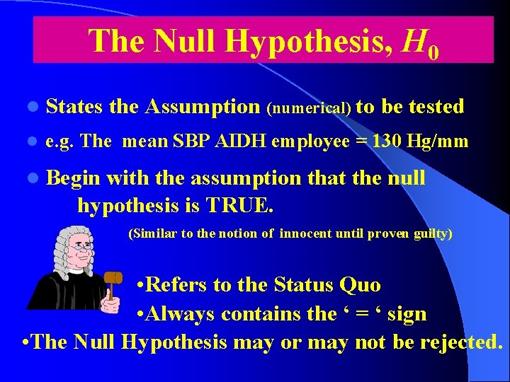
The Null Hypothesis, H 0 l States l the Assumption (numerical) to be tested e. g. The mean SBP AIDH employee = 130 Hg/mm l Begin with the assumption that the null hypothesis is TRUE. (Similar to the notion of innocent until proven guilty) • Refers to the Status Quo • Always contains the ‘ = ‘ sign • The Null Hypothesis may or may not be rejected.

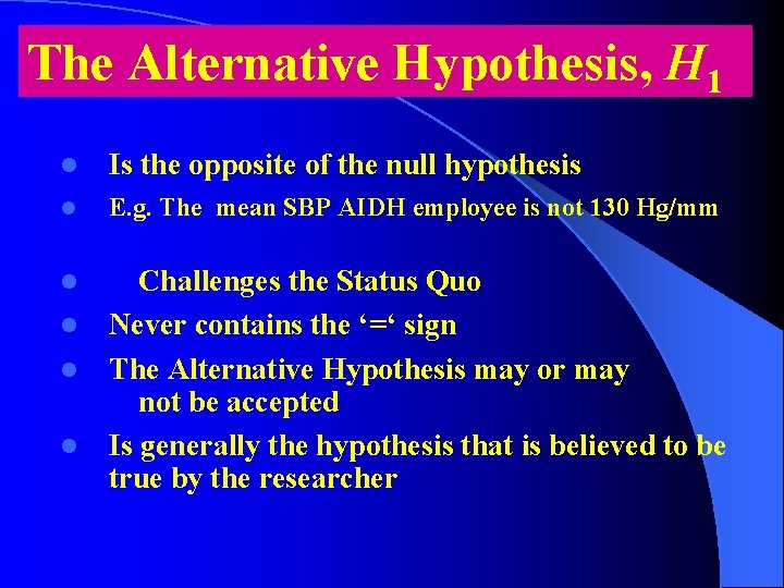
The Alternative Hypothesis, H 1 l Is the opposite of the null hypothesis l E. g. The mean SBP AIDH employee is not 130 Hg/mm Challenges the Status Quo l Never contains the ‘=‘ sign l The Alternative Hypothesis may or may not be accepted l Is generally the hypothesis that is believed to be true by the researcher l

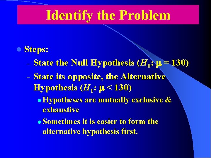
Identify the Problem l Steps: – – State the Null Hypothesis (H 0: m = 130) State its opposite, the Alternative Hypothesis (H 1: m < 130) l Hypotheses are mutually exclusive & exhaustive l Sometimes it is easier to form the alternative hypothesis first.

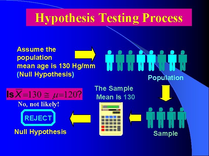
Hypothesis Testing Process Assume the population mean age is 130 Hg/mm (Null Hypothesis) No, not likely! Population The Sample Mean Is 130 REJECT Null Hypothesis Sample

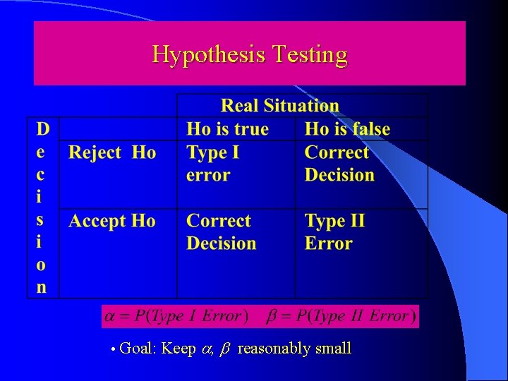
Hypothesis Testing • Goal: Keep a, b reasonably small

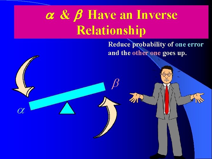
a & b Have an Inverse Relationship Reduce probability of one error and the other one goes up. b a

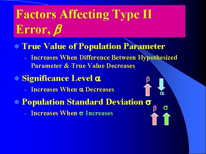
Factors Affecting Type II Error, b l True – Value of Population Parameter Increases When Difference Between Hypothesized Parameter & True Value Decreases l Significance – b Increases When a Decreases l Population – Level a Standard Deviation s Increases When s Increases a b s

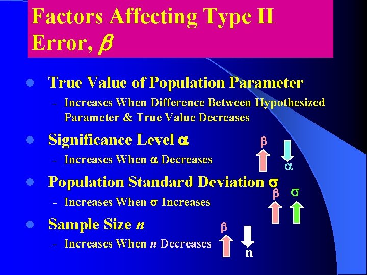
Factors Affecting Type II Error, b l True Value of Population Parameter – l Significance Level a – l b Increases When a Decreases Population Standard Deviation s – l Increases When Difference Between Hypothesized Parameter & True Value Decreases – b s Increases When s Increases Sample Size n Increases When n Decreases a b n

How to choose between Type I and Type II errors l Choice depends on the cost of the error l Choose little type I error when the cost of rejecting the maintained hypothesis or standard treatment is high l Choose large type I error when you have an interest in changing the standard treatment

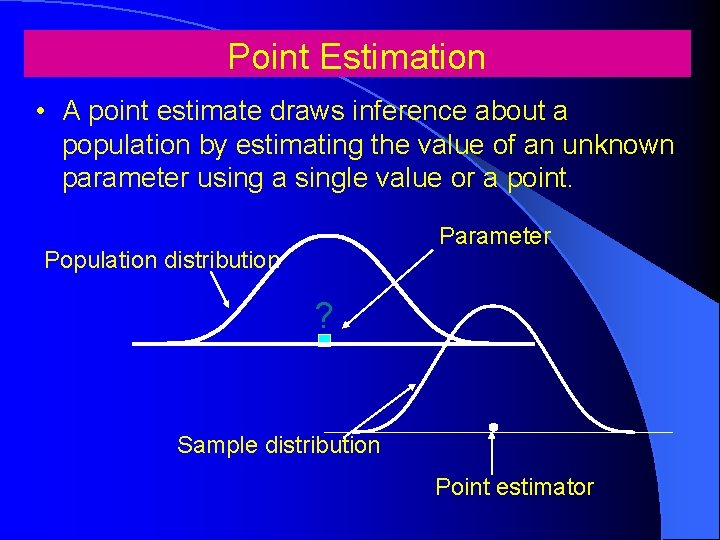
Point Estimation • A point estimate draws inference about a population by estimating the value of an unknown parameter using a single value or a point. Parameter Population distribution ? Sample distribution Point estimator

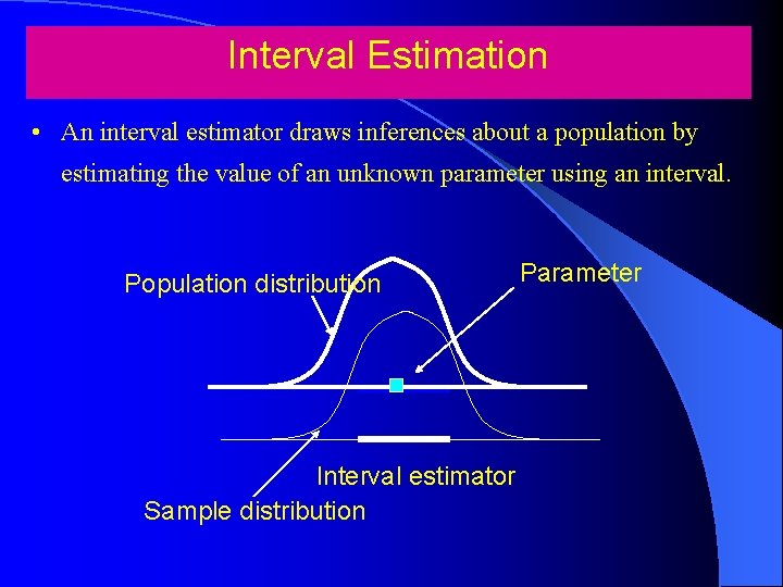
Interval Estimation • An interval estimator draws inferences about a population by estimating the value of an unknown parameter using an interval. Population distribution Interval estimator Sample distribution Parameter

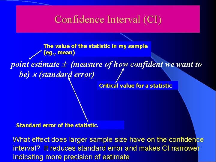
Confidence Interval (CI) The value of the statistic in my sample (eg. , mean) point estimate (measure of how confident we want to be) (standard error) Critical value for a statistic Standard error of the statistic. What effect does larger sample size have on the confidence interval? It reduces standard error and makes CI narrower indicating more precision of estimate

P-Value versus the Confidence Interval l Two main ways to assess study precision and the role of chance in a study. – P value measures ( in probability) the evidence against the null hypothesis. – A p-value of 0. 05 means that in about 5 of 100 experiments, a result would appear significant just by chance (“Type I error”).

P-Value versus the Confidence Interval – A confidence interval (CI) is an interval within which the value of the parameter lies with a specified probability – CI measures the precision of an estimate (when sampling variability is high, the interval is wide to reflect the uncertainty of the estimate) – A 95% CI implies that if one repeats a study 100 times, the true measure of association will lie inside the CI in 95 out of 100 measures. If a parameter does not lie within 95% CI, indicates significance at 5% level of significance

Procedures for sample size calculation l Selection of primary variables of interest and formulation of hypotheses l Information of standard deviation ( if numeric) or proportion (if categorical) l A tolerance level of significance ( ) l Selection of reasonable test statistic l Power or Confidence level l A scientifically or clinically meaning effect/ difference

Useful links for sample size Calculation l 1)http: //hedwig. mgh. harvard. edu/sample_size/size. html l 2)http: //www. stat. uiowa. edu/~rlenth/Power/index. html l 3)http: //cct. jhsph. edu/javamarc/index. htm l 4)http: //stat. ubc. ca/~rollin/stats/ssize/index. html l 5)http: //statpages. org/#Power

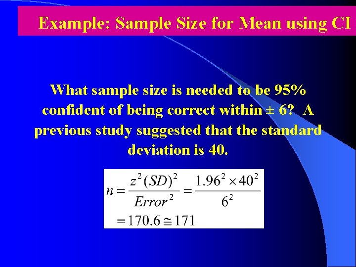
Example: Sample Size for Mean using CI What sample size is needed to be 95% confident of being correct within ± 6? A previous study suggested that the standard deviation is 40.

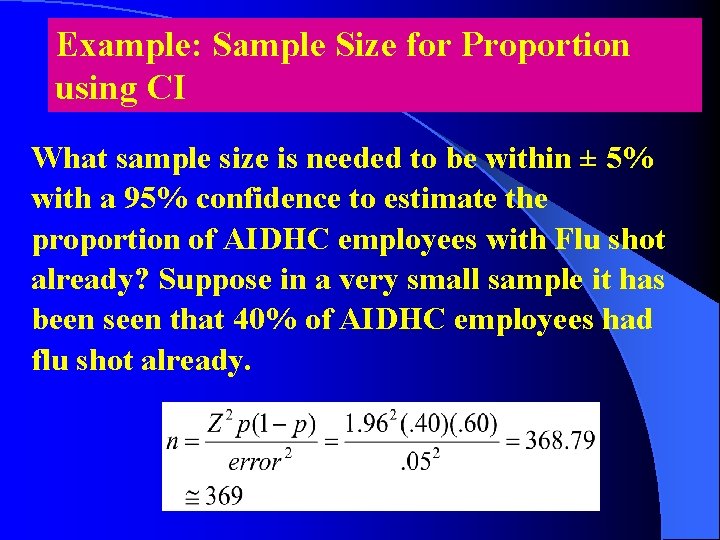
Example: Sample Size for Proportion using CI What sample size is needed to be within ± 5% with a 95% confidence to estimate the proportion of AIDHC employees with Flu shot already? Suppose in a very small sample it has been seen that 40% of AIDHC employees had flu shot already.

Credits l Thanks are due to Faith Goa of the Golden State University for the implied permission to utilize some of the illustrations from their slides on “Fundamentals of Hypothesis Testing” for education purposes only. l Other sources consulted during the preparation of these slides are herein acknowledged as well.

Questions