Research Design Accuracy Precision and Errors Types of

Research Design Accuracy, Precision and Errors

Types of Errors: Type I & II errors drawing the wrong conclusions from our study Type I error: n n A type I error occurs when the null hypothesis is actually true, but was rejected as false by the testing: Rejection of a true null hypothesis. Suppose our null hypothesis is that there is “no wolf present. ” A type I error (or error or false positive) would be “crying wolf” when there is no wolf present. That is, the actual condition was that there was no wolf present; however, the shepherd wrongly indicated there was a wolf present by calling “Wolf!” This is a type I error or false positive error.

Types of Errors: Type I & II errors Type II error: n A type II error occurs when the null hypothesis is actually false, but was accepted as true by the testing: accepting of a false null hypothesis. n A Type II error is committed when we fail to believe a true condition. n Continuing our shepherd and wolf example. Again, our null hypothesis is that there is “no wolf present. ” A type II error (or error or false negative) would be doing nothing (not “crying wolf”) when there is actually a wolf present.

Type I and II errors A patient might take an HIV test, promising a 99. 9% accuracy rate. This means that 1 in every 1000 tests could give a “false positive”, informing a patient that they have the virus, when they do not. Conversely, the test could also show a “false negative” reading, giving an HIV positive patient the all-clear. A Type I error is often referred to as a “false positive”, and is the process of incorrectly rejecting the null hypothesis in favor of the alternative. In the case above, the null hypothesis refers to the natural state of things, stating that the patient is not HIV positive. The alternative hypothesis states that the patient does carry the virus. A Type I error would indicate that the patient has the virus when they do not, a false rejection of the null.

Type II error A Type II error is the opposite of a Type I error and is the false acceptance of the null hypothesis. A Type II error, also known as a false negative, would imply that the patient is free of HIV when they are not, a dangerous diagnosis. In most fields of science, Type II errors are not seen to be as problematic as a Type I error. With the Type II error, a chance to reject the null hypothesis was lost, and no conclusion is inferred from a non-rejected null. The Type I error is more serious, because you have wrongly rejected the null hypothesis. Medicine, however, is one exception; telling a patient that they are free of disease, when they are not, is potentially dangerous.

Decision Reality Drug is effective Drug is not effective Reject H : Decide drug is effective Correct decision Type I error Fail to reject H : Decide drug is not effective Type II error Correct decision

Please identify false positive and false negative statements: v A cancer screening test comes back positive, but you don’t have Type I error the disease. v A new drug shows inhibitory effect on an enzyme, while it has no inhibitory effect. Type I error v A pregnancy test is negative, even though you are in fact Type II error pregnant. v Virus software on your computer incorrectly identifies a harmless program as a malicious one. Type I error v In the blood sample there are some amounts of an analyte, but the biosensor detects no signal of that analyte. Type II error

Sensitivity and specificity n Sensitivity measures the proportion of actual positive which are classified as such (e. g. the percentage of sick people who are identified as having the condition). n In other words, sensitivity of method indicates how responsive it is to a small change in the concentration of an analyte.

§ It can be viewed as the slope of a response curve. § For example, a method having a linear response y = 5 x is two and half times more sensitive than the method exhibiting a linear Response response y = 2 x. Concentration

Sensitivity and specificity n Specificity (selectivity) measures the proportion of negatives who are correctly identified (e. g. the percentage of well people who are identified as not having the condition). n The specificity of a method is a measure of how capable it is of measuring the analyte or variable alone in the presence of other compounds contained in the sample.

Sensitivity and specificity § Sensitivity (i. e. , reliably finding a disease when it is present and avoiding false negatives). § Specificity (i. e. , reliably excluding a disease when it is absent and avoiding false positives). § For example, we want the smoke detectors in our homes to alarm every time there is a fire (i. e. , we want them to be sensitive), but not to be constantly alarm when there is no fire (i. e. , we want them to have specificity)

Sensitivity and specificity n Sensitivity and specificity are usually expressed in percentage. n A theoretical optimal prediction result can achieve 100% sensitive (i. e. predicts all people from a sick population as sick) and 100% specificity (i. e. not predicts any from the healthy population).

False Positives and False Negatives § The negative control (matrix blank) is a sample that closely matches the samples being analyzed with regard to matrix components and is collected to establish the background level (presence and/or absence), of the analyte(s) of interest. § It incorporates all the reagents employed in treating the samples of interest and is subjected to all sample-processing operations. § Its role is to verify that the normal sample matrix does not interfere with or affect the analytical signal. § The negative control may be difficult to obtain because many matrices cannot be closely matched or guaranteed to be free from analytes.

False Positives and False Negatives n A positive control is a quality control sample containing the target analyte(s) and is subjected to all sampleprocessing operations. n The positive control may be a spiked matrix similar to the one being analyzed, or it may be a reference material. n The positive control serves to demonstrate that the analyte of interest would have been detected, if present, at or above a particular concentration.

Analytical blank v It consists of all the reagents or solvents used in an analysis without any of the analyte being present. v A true analytical blank should reflect all the operations to which the analyte in a real sample is subjected. v It is used, for example, in checking that reagents or indicators do not contribute to the volume of titrant required for a titration, including zeroing spectrophotometers or in checking for chromatographic interference.

Limit of detection n This is the smallest amount of an analyte which can be detected by a particular method. It is formally defined as follows: x−x. B=3 s. B where x is the signal from the sample, x. B is the signal from the analytical blank and s. B is the SD of the reading for the analytical blank. n A true limit of detection should reflect all the processes to which the analyte in a real assay is subjected and not be a simple dilution of a pure standard for the analyte until it can no longer be detected. n In the case of chromatographic separations there is usually a constant background reading called the baseline. n In this case, a better definition of the limit of detection is that the analyte should give a signal > three times the standard deviation of the chromatographic baseline within a time range of 0. 5 minutes before and after the peak.

Limit of quantification n The limit of quantification is defined as the smallest amount of analyte which can be quantified reliably, i. e. with an RSD for repeat measurement of <± 20%. n The limit of quantification is defined as: x – x. B = 10 s. B. In this case the analyte should give a peak > ten times the standard deviation of the chromatographic baseline during chromatographic analysis. Exercise: In which of the following cases has the limit of detection been reached? Signal from sample SD Signal from analytical blank Analytical blank SD Abs 0. 0063 0. 0003 0. 0045 0. 0003 Abs 0. 0075 0. 0017 0. 0046 0. 0018 0. 335 ng/ml 0. 045 ng/ml 0. 037 ng/ml

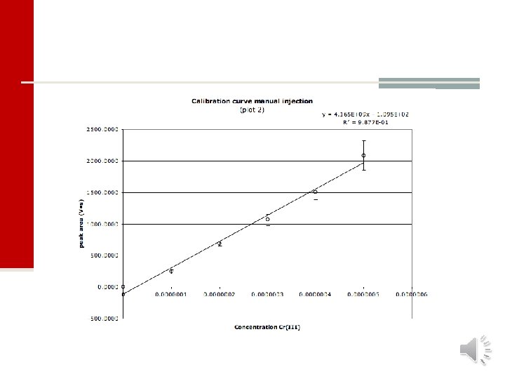
Linearity and calibration curve n Most analytical methods are based on processes where the method produces a response that is linear and which increases or decreases linearly with analyte concentration. The equation of a straight line takes the form: y = a + bx n In analytical chemistry, a calibration curve is a general method for determining the concentration of a substance in an unknown sample by comparing the unknown to a set of standard samples of known concentration. n The calibration curve is a plot of how the “analytical signal” changes with changing concentration of analyte. n For most analyses a plot of response vs. concentration will create a linear relationship. n To find the best-fit straight line we use linear regression analysis. 17200 16. 6 g/ml

Working range n Working range is the concentration or measurement range over which the analytical procedure has been validated. n The analytical procedure should be validated for a working range consistent with its intended purpose. n The low end of the working range depends on the purpose of the analytical procedure.