RESEARCH CORPORATE SIEMENS 1 Combinatorial Calculus in Computer

RESEARCH CORPORATE SIEMENS 1 Combinatorial Calculus in Computer Vision: Formulating and Solving Continuous PDEs on Graphs Leo Grady Department of Imaging and Visualization Siemens Corporate Research

Outline 0) Introduction 1) Theory – Combinatorial and continuous space SIEMENS CORPORATE RESEARCH a) Ingredients of continuous calculus 2 b) Ingredients of combinatorial calculus c) Example 1: Stokes Theorem d) Example 2: Helmholtz decomposition e) Example 3: Laplacian 2) Practice – Segmentation a) Reformulation of the Mumford Shah i) Formulation ii) Results b) Random walker algorithm i) Principle ii) Formulation iii) Results 3) Conclusion

Introduction SIEMENS CORPORATE RESEARCH Bellman (1968): 3 Much of the mathematical analysis that was developed over the eighteenth and nineteenth centuries originated in attempts to circumvent arithmetic. With our ability to do large scale arithmetic. . . we can employ simple, direct methods requiring much less old fashioned mathematical training. . This situation by no mean implies that the mathematician has been dispossessed in mathematical physics. It does signify that he is urgently needed. . to transform the original mathematical problems to the stage where a computer can be utilized profitably by someone with a suitable training. . . Good mathematics, like politics, is the art of the possible. Unfortunately, people quickly forget the origins of a mathematical formulation with the result that it soon acquires a life of its own. Its geneaology then protects it from scrutiny. Because the digital computer has so greatly increased our ability to do arithmetic, it is now imperative that we reexamine all the classical mathematical models of mathematical physics from the standpoints of both physical significance and feasibility of numerical solution. It may well turn out that more realistic descriptions are easier to handle conceptually and computationally with the aid of the computer.

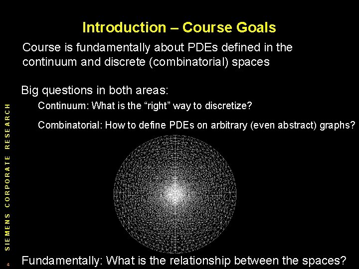
Introduction – Course Goals Course is fundamentally about PDEs defined in the continuum and discrete (combinatorial) spaces Continuum: What is the “right” way to discretize? Combinatorial: How to define PDEs on arbitrary (even abstract) graphs? SIEMENS CORPORATE RESEARCH Big questions in both areas: 4 Fundamentally: What is the relationship between the spaces?

Introduction – Goals SIEMENS CORPORATE RESEARCH Why formulate functionals/PDEs on graphs? 5 1) Remove solution dependency on discretization choices. 2) Offers the arsenal of combinatorial optimization tools to minimize energy (not just gradient descent). 3) Produce a solution with respect to the energy as actually computed. 4) Permit generalization of algorithms to nonuniformly sampled images and even abstract graphs.

Introduction – Goals SIEMENS CORPORATE RESEARCH But, variational/PDE theory is continuous. . . 6 1) Most theorems/concepts persist with an appropriate combinatorial formulation 2) New insights/perspectives on traditional PDEs offered by the combinatorial formulation 3) Traditionally graph based concepts also often benefit from the insight gained by examining the continuous equivalent

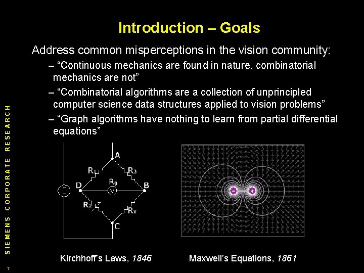
Introduction – Goals – “Continuous mechanics are found in nature, combinatorial mechanics are not” – “Combinatorial algorithms are a collection of unprincipled computer science data structures applied to vision problems” – “Graph algorithms have nothing to learn from partial differential equations” SIEMENS CORPORATE RESEARCH Address common misperceptions in the vision community: 7 Kirchhoff’s Laws, 1846 Maxwell’s Equations, 1861

Introduction - History SIEMENS CORPORATE RESEARCH Representations of space and quantities in space: 8 • 1736 – Euler publishes the solution to the Königsberg bridge problem, defines nodes and edges • 1831 – Geometric representation of 2 D space by complex numbers published by Gauss • 1841 – Incidence matrices defined by Kirchhoff, mapping node potentials to edge flows. Used to define Kirchhoff’s Laws • 1843 – Hamilton formulates quaternions for representation of 3 D space by complex quantities • 1846 – Hamilton coins terms scalar and vector to describe the real and imaginary parts of quaternions, respectively

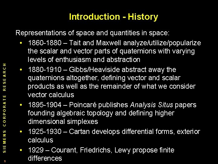
SIEMENS CORPORATE RESEARCH Introduction - History 9 Representations of space and quantities in space: • 1860 1880 – Tait and Maxwell analyze/utilize/popularize the scalar and vector parts of quaternions with varying levels of enthusiasm and abstraction • 1880 1910 – Gibbs/Heaviside abstract away the quaternions altogether, defining vector and scalar products as well as the remainder of what we consider vector calculus • 1895 1904 – Poincaré publishes Analysis Situs papers founding algebraic topology and defining higher dimensional simplexes • 1925 1930 – Cartan develops differential forms, exterior calculus • 1929 – Courant, Friedrichs, Lewy propose finite differences

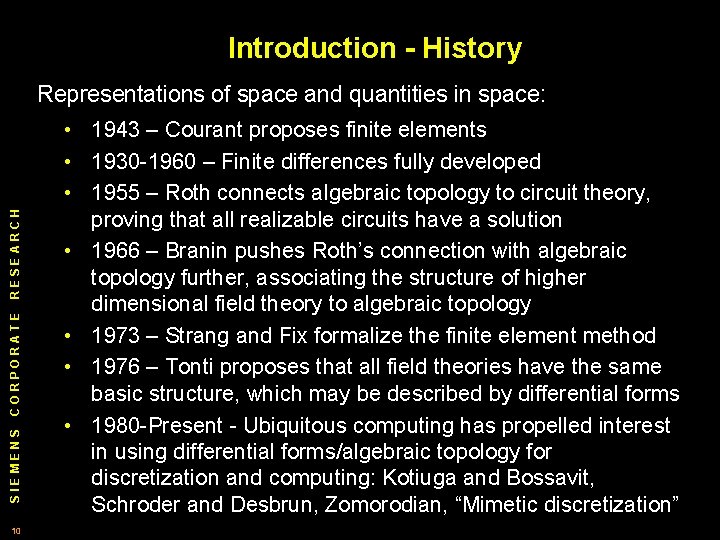
Introduction - History SIEMENS CORPORATE RESEARCH Representations of space and quantities in space: 10 • 1943 – Courant proposes finite elements • 1930 1960 – Finite differences fully developed • 1955 – Roth connects algebraic topology to circuit theory, proving that all realizable circuits have a solution • 1966 – Branin pushes Roth’s connection with algebraic topology further, associating the structure of higher dimensional field theory to algebraic topology • 1973 – Strang and Fix formalize the finite element method • 1976 – Tonti proposes that all field theories have the same basic structure, which may be described by differential forms • 1980 Present Ubiquitous computing has propelled interest in using differential forms/algebraic topology for discretization and computing: Kotiuga and Bossavit, Schroder and Desbrun, Zomorodian, “Mimetic discretization”

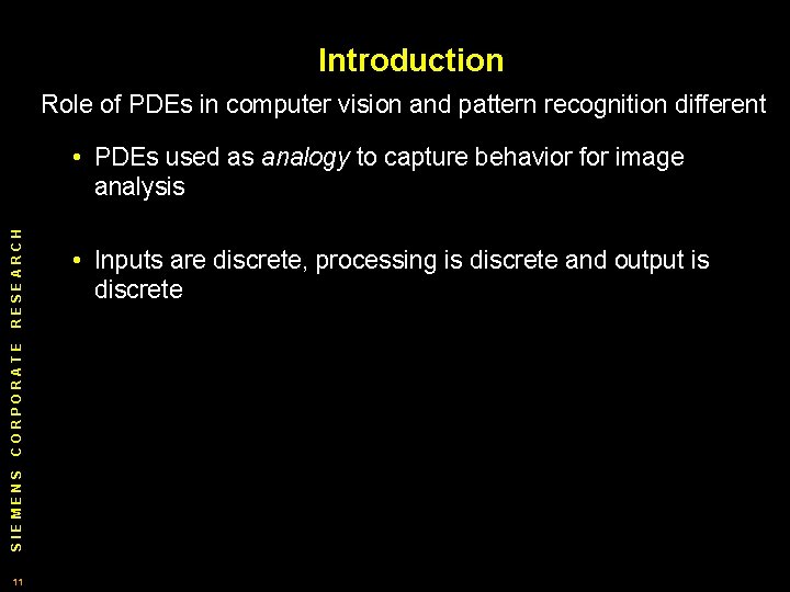
Introduction Role of PDEs in computer vision and pattern recognition different SIEMENS CORPORATE RESEARCH • PDEs used as analogy to capture behavior for image analysis 11 • Inputs are discrete, processing is discrete and output is discrete

Outline 0) Introduction 1) Theory – Combinatorial and continuous space SIEMENS CORPORATE RESEARCH a) Ingredients of continuous calculus 12 b) Ingredients of combinatorial calculus c) Example 1: Stokes Theorem d) Example 2: Helmholtz decomposition e) Example 3: Laplacian 2) Practice – Segmentation a) Reformulation of the Mumford Shah i) Formulation ii) Results b) Random walker algorithm i) Principle ii) Formulation iii) Results 3) Conclusion

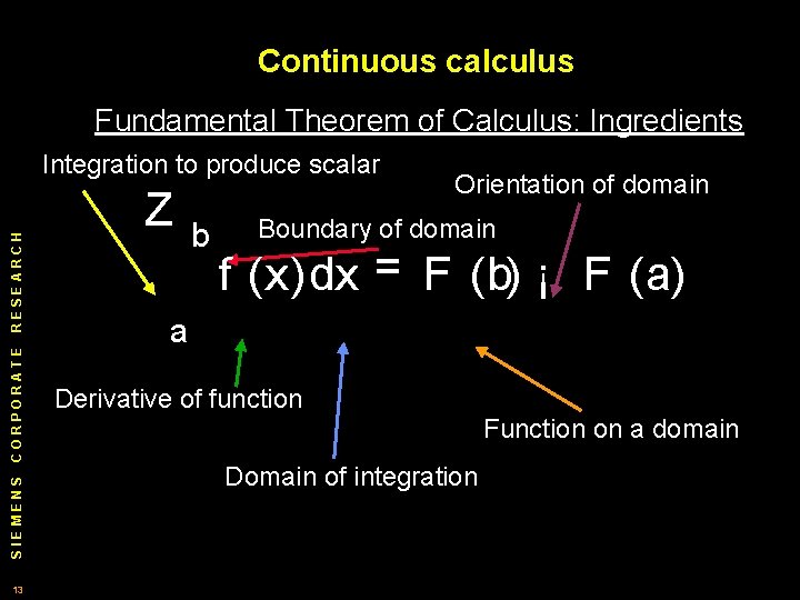
Continuous calculus Fundamental Theorem of Calculus: Ingredients SIEMENS CORPORATE RESEARCH Integration to produce scalar 13 Z b Orientation of domain Boundary of domain f (x)dx = F (b) ¡ F (a) a Derivative of function Function on a domain Domain of integration

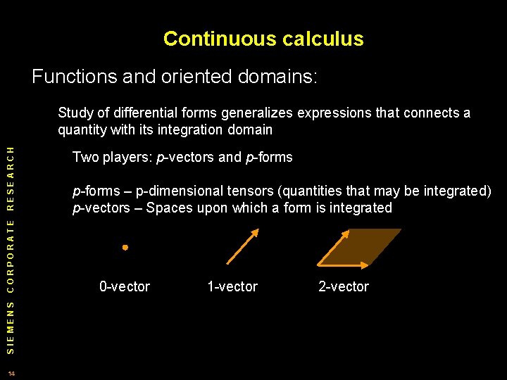
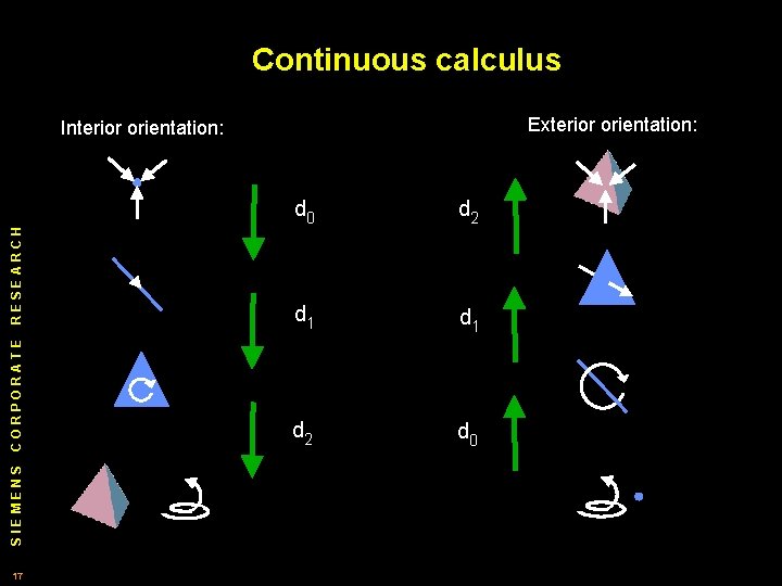
Continuous calculus Functions and oriented domains: SIEMENS CORPORATE RESEARCH Study of differential forms generalizes expressions that connects a quantity with its integration domain 14 Two players: p vectors and p forms p-forms – p dimensional tensors (quantities that may be integrated) p vectors – Spaces upon which a form is integrated 0 vector 1 vector 2 vector

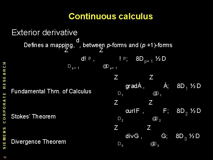
Continuous calculus Exterior derivative d Defines a mapping, , between p forms and (p +1) forms SIEMENS CORPORATE RESEARCH Z 15 Z d! Dp+ p 1 , ! p; @D p + 8 D p+ 1 ½ D 1 Z Fundamental Thm. of Calculus Z gradÁ , curl. F , 8 D 2 ½ D G; 8 D 3 ½ D @D 2 Z div. G , D 3 F; Z Z Divergence Theorem 8 D 1 ½ D @D 1 Z Stokes’ Theorem Á; @D 3

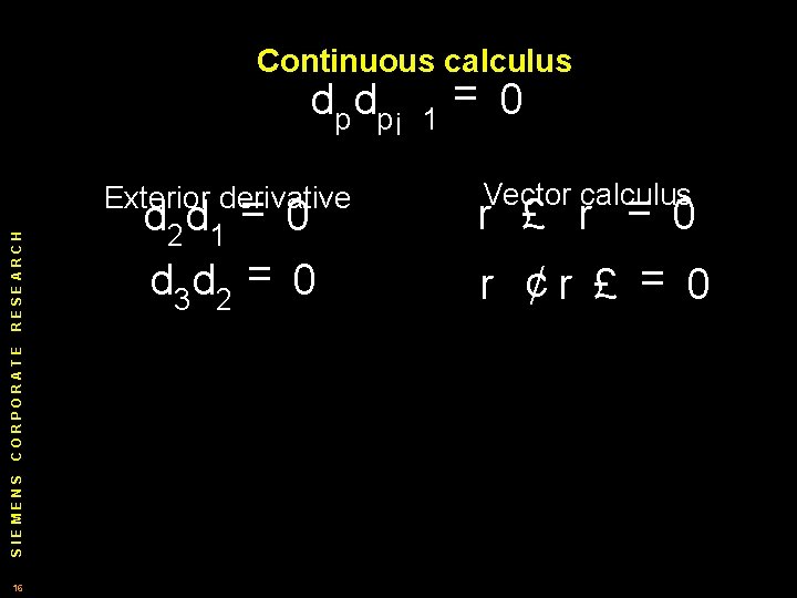
Continuous calculus SIEMENS CORPORATE RESEARCH dp dp¡ 16 Exterior derivative d 2 d 1 = 0 d 3 d 2 = 0 1 = 0 Vector calculus r £ r = 0 r ¢r £ = 0

Continuous calculus Exterior orientation: SIEMENS CORPORATE RESEARCH Interior orientation: 17 d 0 d 2 d 1 d 2 d 0

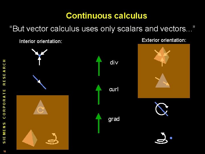
Continuous calculus “But vector calculus uses only scalars and vectors. . . ” Exterior orientation: SIEMENS CORPORATE RESEARCH Interior orientation: 18 div curl grad

Outline 0) Introduction 1) Theory – Combinatorial and continuous space SIEMENS CORPORATE RESEARCH a) Ingredients of continuous calculus 19 b) Ingredients of combinatorial calculus c) Example 1: Stokes Theorem d) Example 2: Helmholtz decomposition e) Example 3: Laplacian 2) Practice – Segmentation a) Reformulation of the Mumford Shah i) Formulation ii) Results b) Random walker algorithm i) Principle ii) Formulation iii) Results 3) Conclusion

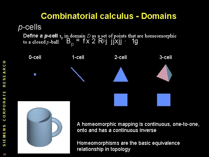
Combinatorial calculus - Domains p cells Define a p-cell τp in domain D as a set of points that are homeomorphic to a closed p-ball B p = f x 2 Rp j jjxjj · 1 g 1 cell 2 cell 3 cell SIEMENS CORPORATE RESEARCH 0 cell 20 A homeomorphic mapping is continuous, one to one, onto and has a continuous inverse Homeomorphisms are the basic equivalence relationship in topology

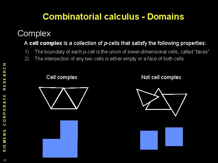
Combinatorial calculus - Domains Complex A cell complex is a collection of p cells that satisfy the following properties: SIEMENS CORPORATE RESEARCH 1) 2) 21 The boundary of each p-cell is the union of lower dimensional cells, called “faces” The intersection of any two cells is either empty or a face of both cells Cell complex Not cell complex

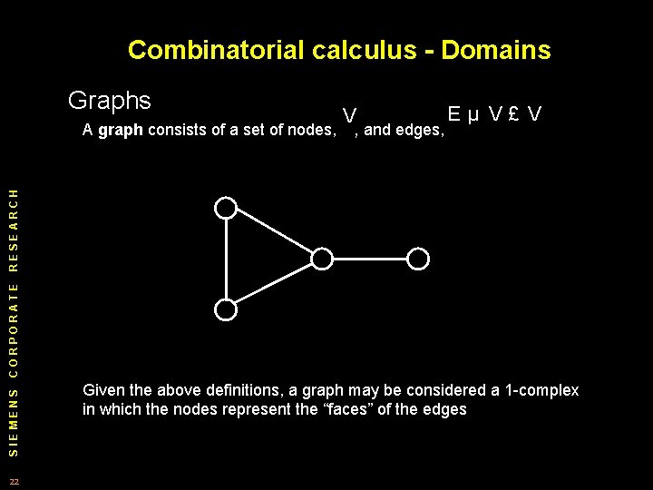
Combinatorial calculus - Domains Graphs , and edges, Eµ V£ V SIEMENS CORPORATE RESEARCH A graph consists of a set of nodes, V 22 Given the above definitions, a graph may be considered a 1 complex in which the nodes represent the “faces” of the edges

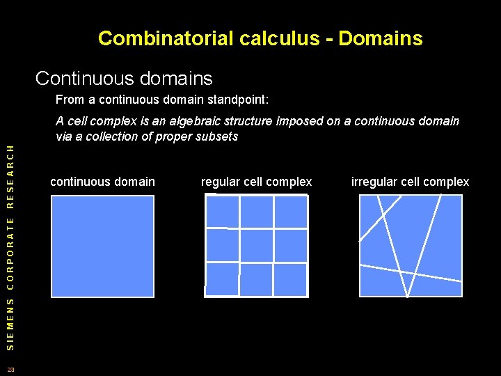
Combinatorial calculus - Domains Continuous domains From a continuous domain standpoint: SIEMENS CORPORATE RESEARCH A cell complex is an algebraic structure imposed on a continuous domain via a collection of proper subsets 23 continuous domain regular cell complex irregular cell complex

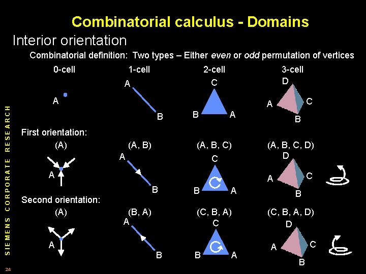
Combinatorial calculus - Domains Interior orientation Combinatorial definition: Two types – Either even or odd permutation of vertices 0 cell 1 cell 2 cell C SIEMENS CORPORATE RESEARCH A 24 3 cell D A B First orientation: (A) (A, B) B A (A, B, C) A C A Second orientation: (A) A C A B (A, B, C, D) D C A B (B, A) A B A (C, B, A) C B B A B (C, B, A, D) D C A B

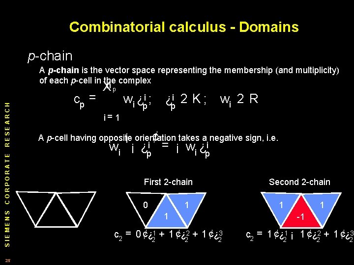
Combinatorial calculus - Domains SIEMENS CORPORATE RESEARCH p chain 25 A p-chain is the vector space representing the membership (and multiplicity) of each p cell in the complex Xn p cp = wi ¿pi ; ¿pi 2 K ; wi 2 R i= 1 ¡ orientation ¢ takes a negative sign, i. e. A p cell having opposite wi ¡ ¿pi = ¡ wi ¿pi First 2 chain 0 1 Second 2 chain 1 1 1 1 c 2 = 0 ¢¿ 21 + 1 ¢¿ 22 + 1 ¢¿ 23 c 2 = 1 ¢¿ 21 ¡ 1 ¢¿ 22 + 1 ¢¿ 23

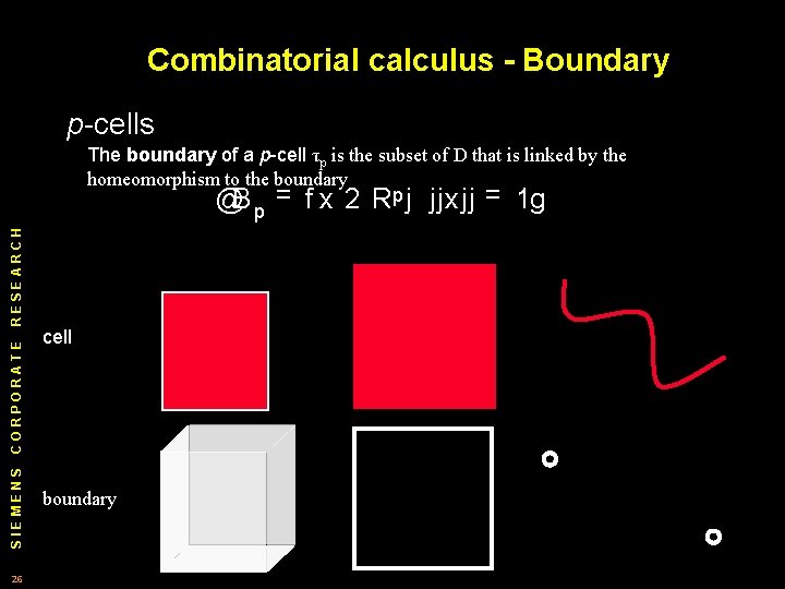
Combinatorial calculus - Boundary p cells SIEMENS CORPORATE RESEARCH The boundary of a p cell τp is the subset of D that is linked by the homeomorphism to the boundary @B p = f x 2 Rp j jjxjj = 1 g 26 cell boundary

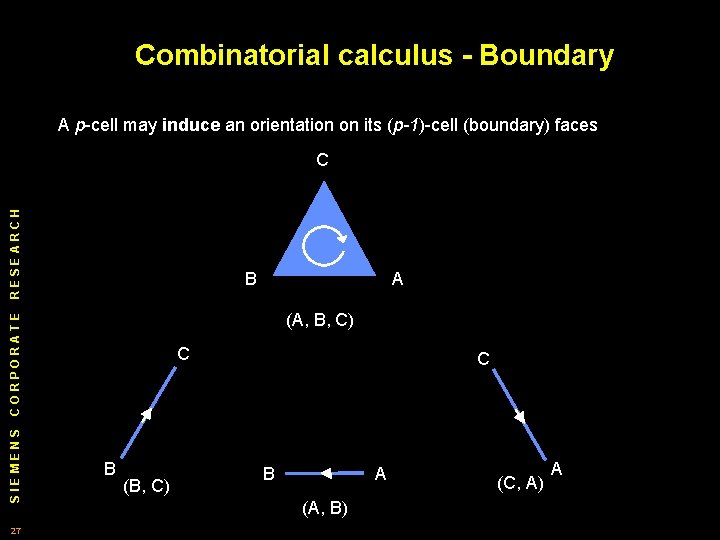
Combinatorial calculus - Boundary A p cell may induce an orientation on its (p-1) cell (boundary) faces RESEARCH C B (A, B, C) CORPORATE SIEMENS 27 A C B (B, C) C B A (A, B) (C, A) A

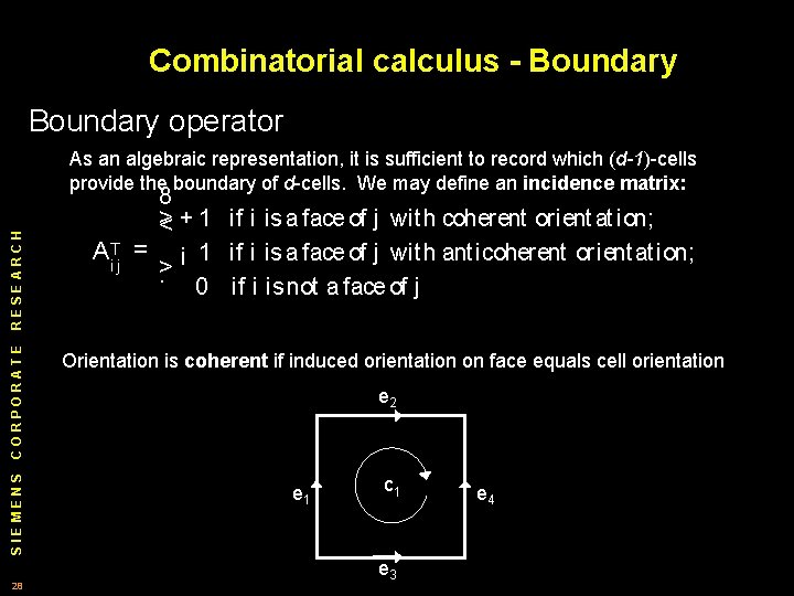
Combinatorial calculus - Boundary operator SIEMENS CORPORATE RESEARCH As an algebraic representation, it is sufficient to record which (d-1) cells provide the boundary of d cells. We may define an incidence matrix: 28 A i. Tj 8 > < + 1 if i is a faceof j wit h coherent orient at ion; = ¡ 1 if i is a faceof j wit h anticoherent orient at ion; > : 0 if i is not a faceof j Orientation is coherent if induced orientation on face equals cell orientation e 2 e 1 c 1 e 3 e 4

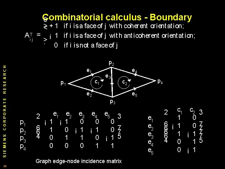
Combinatorial calculus - Boundary 8 A i. Tj p 2 RESEARCH CORPORATE SIEMENS > < + 1 if i is a faceof j wit h coherent orient at ion; = ¡ 1 if i is a faceof j wit h anticoherent orient at ion; > : 0 if i is not a faceof j e 1 c 1 p 1 e 3 e 2 p 4 c 2 e 5 p 3 p 1 p 2 p 3 p 4 e 1 2 ¡ 1 ¡ 6 1 6 4 0 0 e 2 e 3 e 4 e 5 3 1 0 0 ¡ 1 0 7 7 1 1 0 ¡ 1 5 0 0 1 1 Graph edge node incidence matrix 29 e 4 e 1 e 2 e 3 e 4 e 5 c 1 c 2 1 0 6 ¡ 1 0 6 6 1 ¡ 1 6 4 0 1 0 ¡ 1 2 3 7 7 5

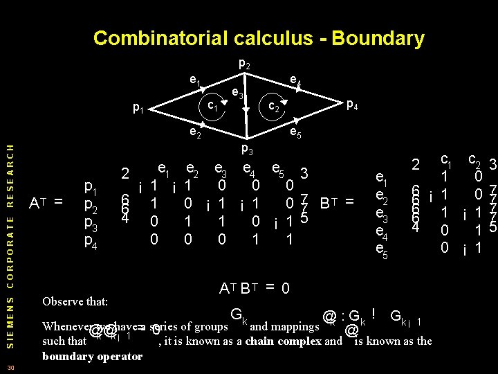
Combinatorial calculus - Boundary p 2 e 1 c 1 p 1 e 4 e 3 SIEMENS CORPORATE RESEARCH e 2 30 p 4 c 2 e 5 p 3 AT = p 1 p 2 p 3 p 4 Observe that: e 1 2 ¡ 1 ¡ 6 1 6 4 0 0 e 2 e 3 e 4 e 5 3 1 0 0 0 T 0 ¡ 1 0 7 7 B = 1 1 0 ¡ 1 5 0 0 1 1 e 2 e 3 e 4 e 5 c 1 c 2 1 0 6 ¡ 1 0 6 6 1 ¡ 1 6 4 0 1 0 ¡ 1 2 AT B T = 0 Gk @k : Gk ! Gk ¡ and mappings @ Whenever@ we have=a series 0 of groups k@ k¡ 1 such that , it is known as a chain complex and boundary operator 1 is known as the 3 7 7 5

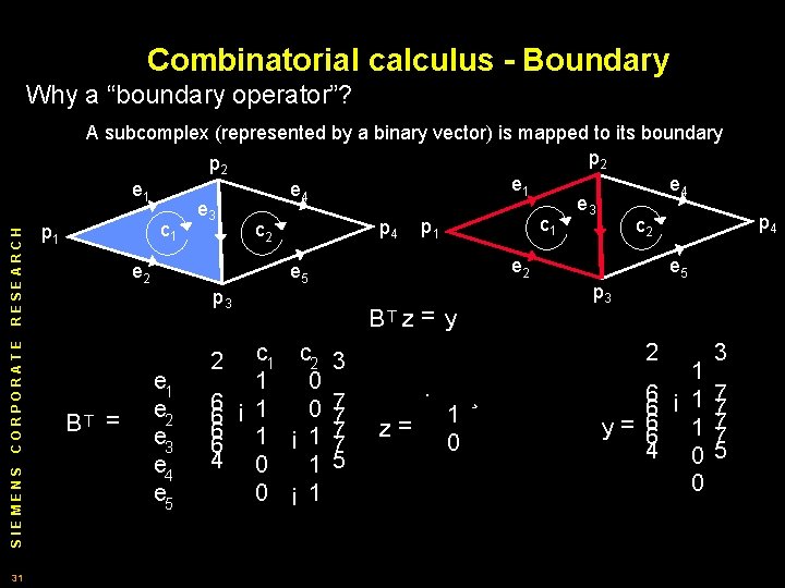
Combinatorial calculus - Boundary SIEMENS CORPORATE RESEARCH Why a “boundary operator”? 31 p 1 A subcomplex (represented by a binary vector) is mapped to its boundary p 2 e 1 e 4 e 3 c 1 c 2 p 4 p 1 c 2 e 2 e 5 p 3 BT = e 1 e 2 e 3 e 4 e 5 c 1 c 2 1 0 6 ¡ 1 0 6 6 1 ¡ 1 6 4 0 1 0 ¡ 1 2 p 3 BT z = y 2 3 7 7 5 e 5 · z= 1 0 ¸ 1 6 ¡ 1 6 y= 6 6 1 4 0 0 3 7 7 5 p 4

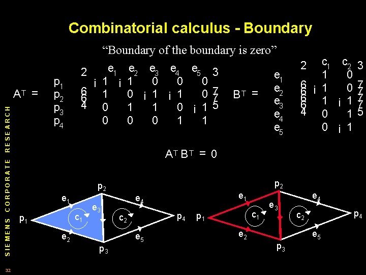
Combinatorial calculus - Boundary “Boundary of the boundary is zero” RESEARCH AT = e 2 e 3 e 4 e 5 3 1 0 0 ¡ 1 0 7 7 1 1 0 ¡ 1 5 0 0 1 1 BT = e 1 e 2 e 3 e 4 e 5 3 7 7 5 AT B T = 0 CORPORATE SIEMENS 32 p 1 p 2 p 3 p 4 e 1 ¡ 6 1 6 4 0 0 2 c 1 c 2 1 0 6 ¡ 1 0 6 6 1 ¡ 1 6 4 0 1 0 ¡ 1 2 p 2 e 1 c 1 p 1 e 3 e 2 p 4 c 2 e 5 p 3 e 1 e 4 c 1 p 1 e 3 e 2 e 4 p 4 c 2 e 5 p 3

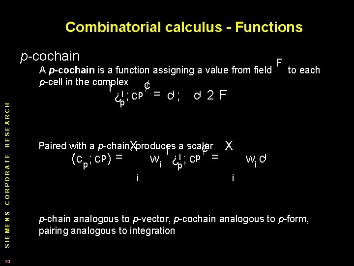
Combinatorial calculus - Functions p cochain SIEMENS CORPORATE RESEARCH A p-cochain is a function assigning a value from field p cell in the complex ¡ ¢ 33 ¿pi ; cp = ci ; wi ¿pi ; cp = i to each ci 2 F Paired with a p chain, Xproduces ¡ a scalar ¢ (cp ; cp ) = F X wi ci i p chain analogous to p vector, p cochain analogous to p form, pairing analogous to integration

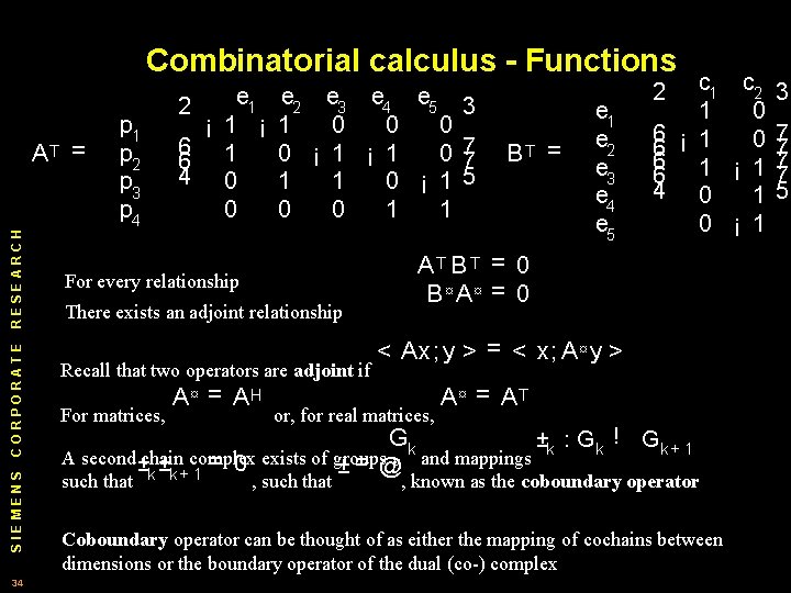
Combinatorial calculus - Functions SIEMENS CORPORATE RESEARCH AT 34 = p 1 p 2 p 3 p 4 e 1 2 ¡ 1 ¡ 6 1 6 4 0 0 e 2 e 3 e 4 e 5 3 1 0 0 ¡ 1 0 7 7 1 1 0 ¡ 1 5 0 0 1 1 For every relationship There exists an adjoint relationship Recall that two operators are adjoint if For matrices, A¤ = AH BT = e 1 e 2 e 3 e 4 e 5 c 1 c 2 1 0 6 ¡ 1 0 6 6 1 ¡ 1 6 4 0 1 0 ¡ 1 2 AT B T = 0 B ¤A¤ = 0 < Ax; y > = < x; A ¤ y > or, for real matrices, A¤ = AT Gk ±k : Gk ! Gk + 1 A second ±chain complex exists of groups ¤ and mappings = = ± 0 ± @ k k+ 1 such that , known as the coboundary operator Coboundary operator can be thought of as either the mapping of cochains between dimensions or the boundary operator of the dual (co-) complex 3 7 7 5

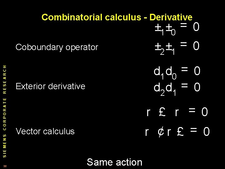
Combinatorial calculus - Derivative SIEMENS CORPORATE RESEARCH Coboundary operator 35 ± 1 ± 0 = 0 ± 2 ± 1 = 0 d 1 d 0 = 0 d 2 d 1 = 0 Exterior derivative r £ r = 0 r ¢r £ = 0 Vector calculus Same action

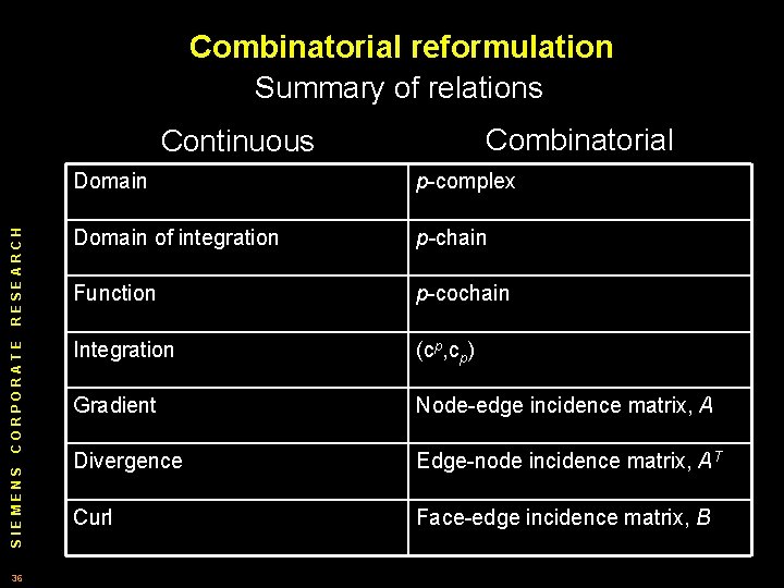
Combinatorial reformulation Summary of relations Combinatorial p complex RESEARCH Domain of integration p-chain Function p cochain Integration (cp, cp) Gradient Node edge incidence matrix, A Divergence Edge node incidence matrix, AT Curl Face edge incidence matrix, B SIEMENS Domain CORPORATE Continuous 36

Outline 0) Introduction 1) Theory – Combinatorial and continuous space SIEMENS CORPORATE RESEARCH a) Ingredients of continuous calculus 37 b) Ingredients of combinatorial calculus c) Example 1: Stokes Theorem d) Example 2: Helmholtz decomposition e) Example 3: Laplacian 2) Practice – Segmentation a) Reformulation of the Mumford Shah i) Formulation ii) Results b) Random walker algorithm i) Principle ii) Formulation iii) Results 3) Conclusion

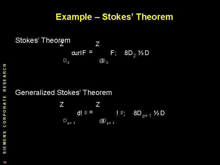
Example – Stokes’ Theorem Z Z SIEMENS CORPORATE RESEARCH curl. F = 38 D 2 F; @D 2 8 D 2 ½ D Generalized Stokes’ Theorem Z Z d! Dp+ 1 p = ! p; @D p + 1 8 D p+ 1 ½ D

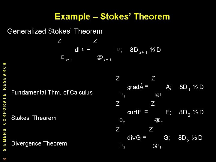
Example – Stokes’ Theorem Generalized Stokes’ Theorem Z Z d! SIEMENS CORPORATE RESEARCH Dp+ 39 p = 1 ! p; @D p + 8 D p+ 1 ½ D 1 Z Fundamental Thm. of Calculus Z gradÁ = curl. F = 8 D 2 ½ D G; 8 D 3 ½ D @D 2 Z div. G = D 3 F; Z Z Divergence Theorem 8 D 1 ½ D @D 1 Z Stokes’ Theorem Á; @D 3

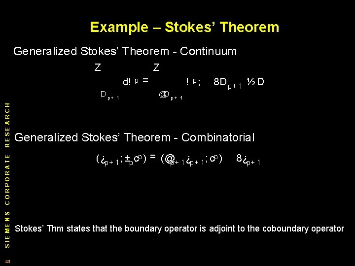
Example – Stokes’ Theorem Generalized Stokes’ Theorem Continuum Z Z d! SIEMENS CORPORATE RESEARCH Dp+ 40 1 p = ! p; @D p + 8 D p+ 1 ½ D 1 Generalized Stokes’ Theorem Combinatorial (¿p+ 1 ; ±p cp ) = (@p+ 1 ¿p+ 1 ; cp ) 8¿p+ 1 Stokes’ Thm states that the boundary operator is adjoint to the coboundary operator

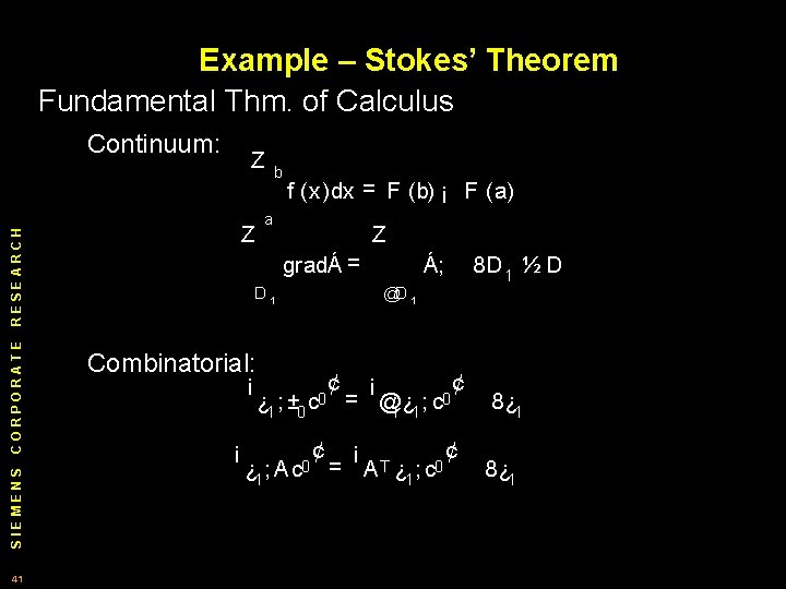
Example – Stokes’ Theorem Fundamental Thm. of Calculus Continuum: Z f (x)dx = F (b) ¡ F (a) a Z RESEARCH CORPORATE SIEMENS 41 b Z gradÁ = @D 1 Combinatorial: ¡ ¡ ¿ 1 ; ± 0 ¿ 1 8 D 1 ½ D Á; c 0 ; Ac 0 ¢ ¢ ¡ = @1 ¿ 1 ; c 0 ¢ ¡ ¢ = A T ¿ 1 ; c 0 8¿ 1

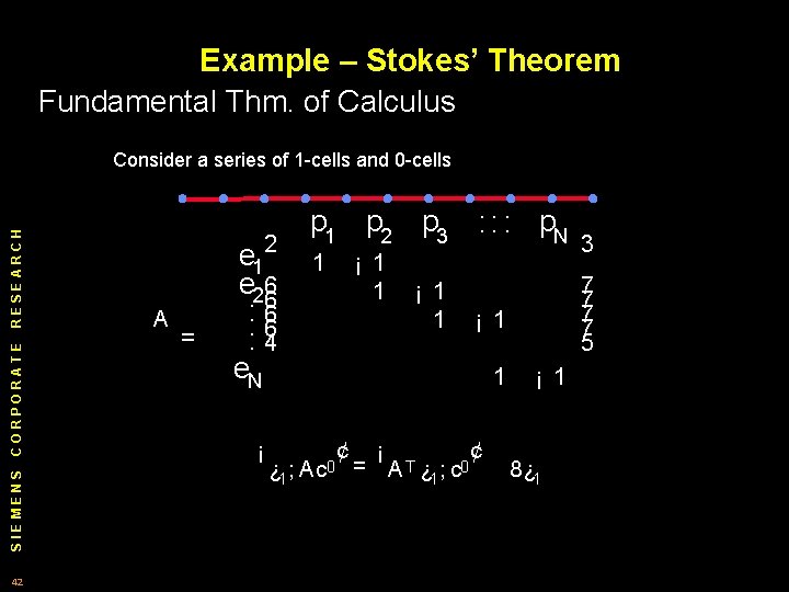
Example – Stokes’ Theorem Fundamental Thm. of Calculus SIEMENS CORPORATE RESEARCH Consider a series of 1 cells and 0 cells 42 A = e 12 e 266 : 4 e. N ¡ ¿ 1 p 2 p 3 : : : p. N 1 ¡ 1 1 ; Ac 0 ¢ = ¡ A T ¿ 1 ; c 0 7 7 5 ¡ 1 1 ¢ 3 ¡ 1 8¿ 1

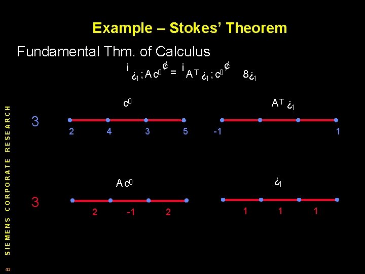
Example – Stokes’ Theorem Fundamental Thm. of Calculus SIEMENS CORPORATE RESEARCH ¡ 43 ¢ ¡ ¿ 1 ; Ac 0 = A T ¿ 1 ; c 0 ¢ 8¿ 1 c 0 3 2 4 A T ¿ 1 3 5 1 1 ¿ 1 Ac 0 3 2 1 2 1 1 1

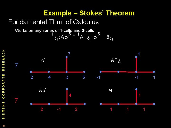
Example – Stokes’ Theorem Fundamental Thm. of Calculus Works on any series of 1 cells and 0 cells SIEMENS CORPORATE RESEARCH ¡ 44 ¿ 1 ; Ac 0 ¢ = ¡ A T ¿ 1 ; c 0 ¢ 8¿ 1 1 7 c 0 7 2 A T ¿ 1 4 3 1 1 1 ¿ 1 Ac 0 4 7 2 5 1 1 2 1 1 1

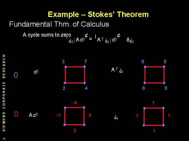
Example – Stokes’ Theorem Fundamental Thm. of Calculus A cycle sums to zero ¡ 3 0 SIEMENS 45 ¢ = ¡ A T ¿ 1 ; c 0 ¢ 8¿ 1 7 2 4 4 0 Ac 0 0 0 A T ¿ 1 c 0 CORPORATE RESEARCH ¿ 1 ; Ac 0 1 3 1 2 ¿ 1 1

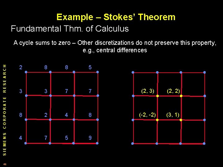
Example – Stokes’ Theorem Fundamental Thm. of Calculus SIEMENS CORPORATE RESEARCH A cycle sums to zero – Other discretizations do not preserve this property, e. g. , central differences 46 2 8 8 5 3 3 7 7 (2, 3) (2, 2) 8 2 4 8 ( 2, 2) (3, 1) 4 7 5 9

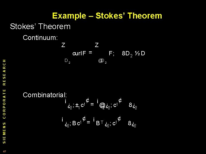
Example – Stokes’ Theorem Continuum: Z Z curl. F = SIEMENS CORPORATE RESEARCH D 2 47 @D 2 Combinatorial: ¡ ¡ ¿ 2 ; ± 1 ¿ 2 8 D 2 ½ D F; c 1 ; B c 1 ¢ ¢ ¡ = @2 ¿ 2 ; c 1 ¢ ¡ ¢ = B T ¿ 2 ; c 1 8¿ 2

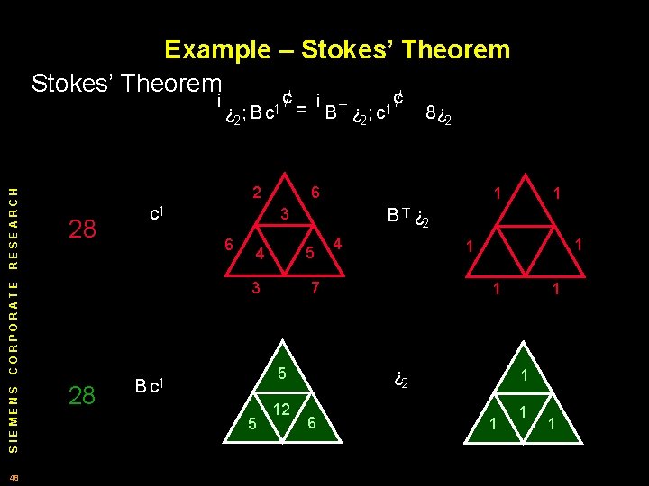
Example – Stokes’ Theorem¡ ¢ 2 28 c 1 3 SIEMENS 48 28 1 5 5 4 1 1 7 12 1 B T ¿ 2 5 4 B c 1 8¿ 2 6 3 6 CORPORATE RESEARCH ¿ 2 ; B c 1 = B T ¿ 2 ; c 1 1 ¿ 2 6 1 1 1

Outline 0) Introduction 1) Theory – Combinatorial and continuous space SIEMENS CORPORATE RESEARCH a) Ingredients of continuous calculus 49 b) Ingredients of combinatorial calculus c) Example 1: Stokes Theorem d) Example 2: Helmholtz decomposition e) Example 3: Laplacian 2) Practice – Segmentation a) Reformulation of the Mumford Shah i) Formulation ii) Results b) Random walker algorithm i) Principle ii) Formulation iii) Results 3) Conclusion

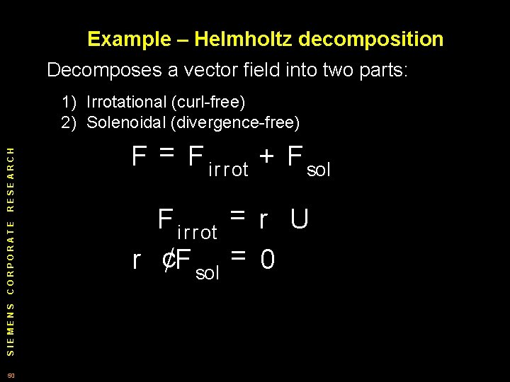
Example – Helmholtz decomposition Decomposes a vector field into two parts: SIEMENS CORPORATE RESEARCH 1) Irrotational (curl free) 2) Solenoidal (divergence free) 50 F = F i r r ot + F sol F i r r ot = r U r ¢F sol = 0

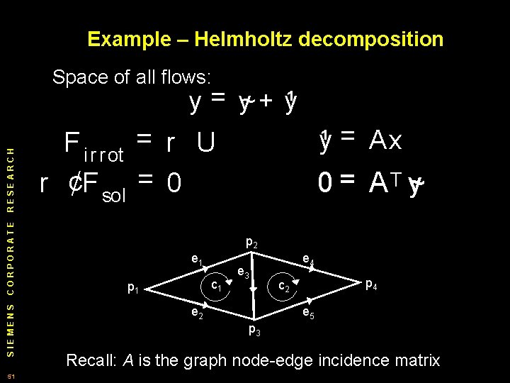
Example – Helmholtz decomposition Space of all flows: SIEMENS CORPORATE RESEARCH y = y~ + y¹ 51 y¹ = Ax F i r r ot = r U r ¢F sol = 0 0 = A T y~ p 2 e 1 c 1 p 1 e 3 e 2 e 4 p 4 c 2 e 5 p 3 Recall: A is the graph node edge incidence matrix

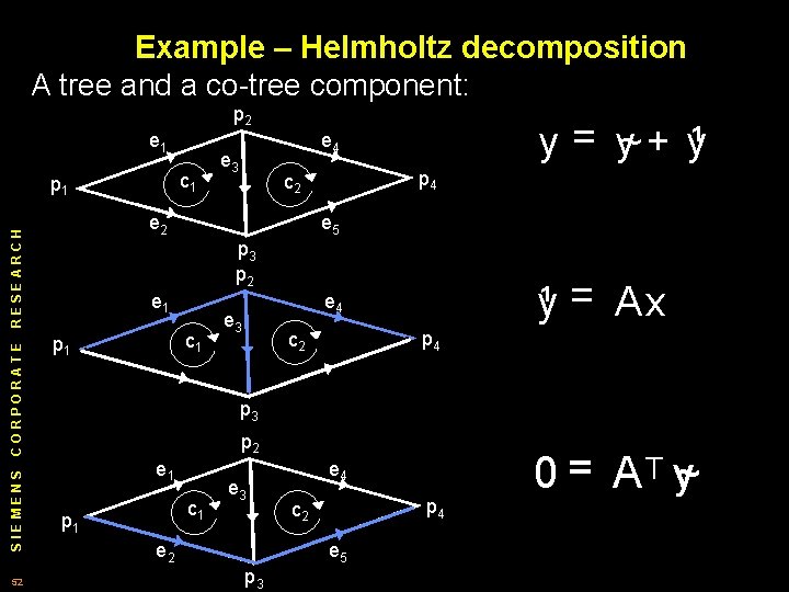
Example – Helmholtz decomposition A tree and a co tree component: p 2 e 1 c 1 p 1 e 3 p 4 c 2 e 2 RESEARCH CORPORATE SIEMENS 52 y = y~ + y¹ e 4 e 5 p 3 p 2 e 1 c 1 p 1 y¹ = Ax e 4 e 3 p 4 c 2 p 3 p 2 e 1 c 1 p 1 e 3 e 2 e 4 p 4 c 2 e 5 p 3 0 = A T y~

Outline 0) Introduction 1) Theory – Combinatorial and continuous space SIEMENS CORPORATE RESEARCH a) Ingredients of continuous calculus 53 b) Ingredients of combinatorial calculus c) Example 1: Stokes Theorem d) Example 2: Helmholtz decomposition e) Example 3: Laplacian 2) Practice – Segmentation a) Reformulation of the Mumford Shah i) Formulation ii) Results b) Random walker algorithm i) Principle ii) Formulation iii) Results 3) Conclusion

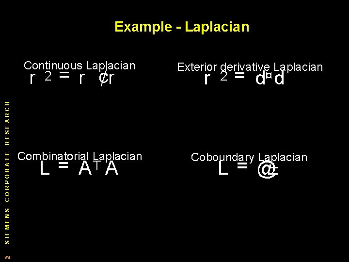
Example - Laplacian Continuous Laplacian Exterior derivative Laplacian Combinatorial Laplacian Coboundary Laplacian 2 = r ¢r r 2 = d¤ d SIEMENS CORPORATE RESEARCH r 54 L = AT A L = @±

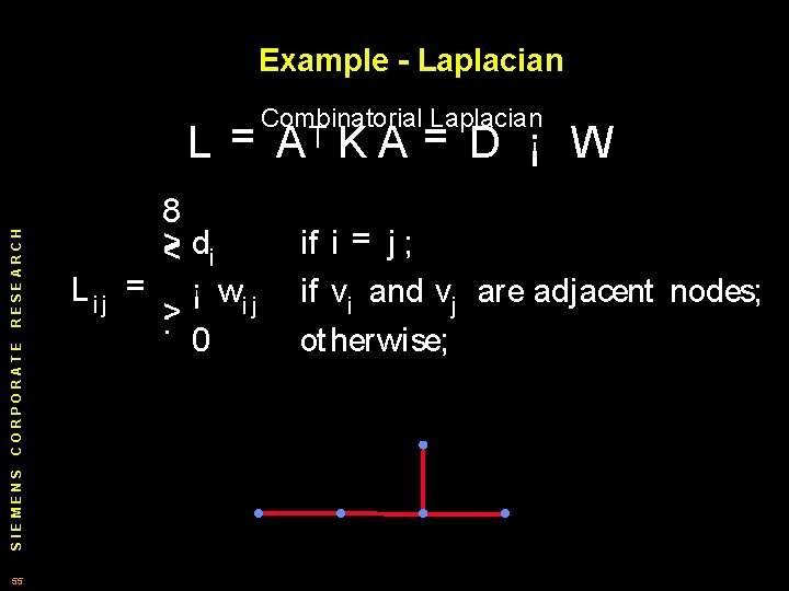
Example - Laplacian Combinatorial Laplacian SIEMENS CORPORATE RESEARCH L = AT K A = D ¡ W 55 Lij 8 > < di = ¡ w ij > : 0 if i = j ; if vi and vj are adjacent nodes; ot herwise;

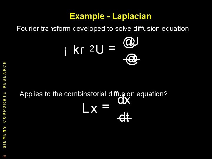
Example - Laplacian SIEMENS CORPORATE RESEARCH Fourier transform developed to solve diffusion equation 56 U @ ¡ kr 2 U = @t Applies to the combinatorial diffusion equation? dx Lx = dt

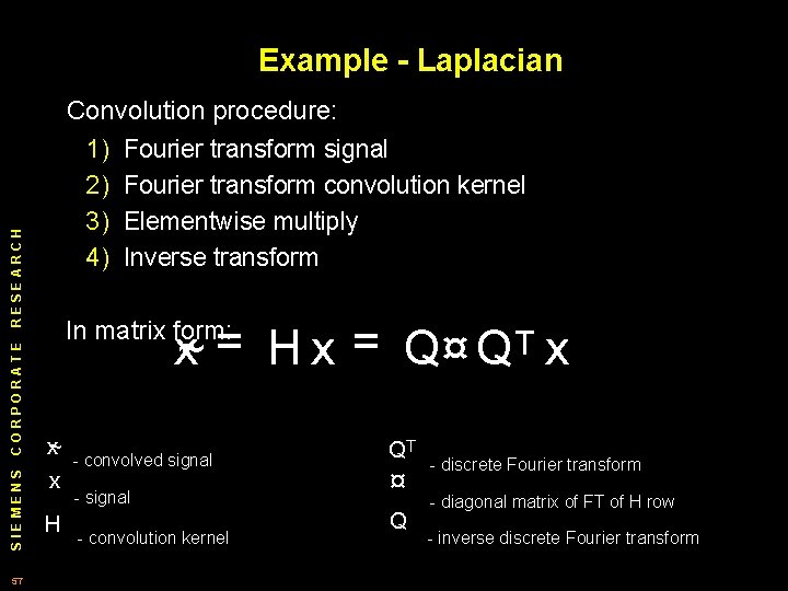
Example - Laplacian SIEMENS CORPORATE RESEARCH Convolution procedure: 1) Fourier transform signal 2) Fourier transform convolution kernel 3) Elementwise multiply 4) Inverse transform 57 x~ = H x = Q¤ QT x In matrix form: x~ x H convolved signal convolution kernel QT ¤ Q discrete Fourier transform diagonal matrix of FT of H row inverse discrete Fourier transform

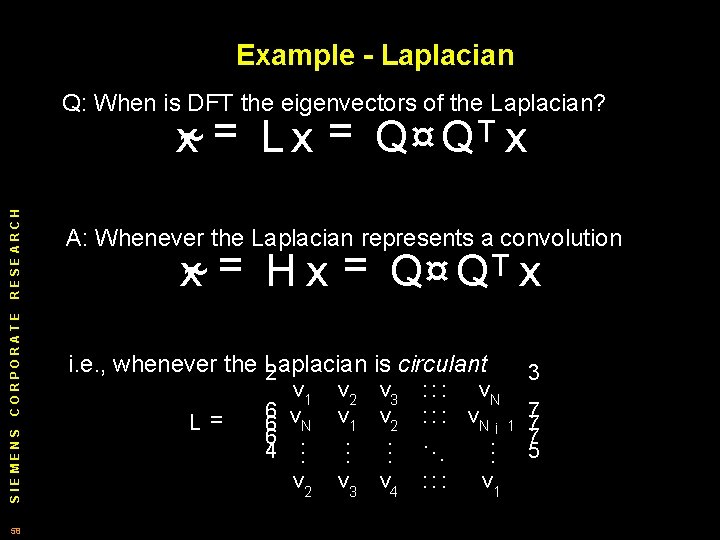
Example - Laplacian Q: When is DFT the eigenvectors of the Laplacian? SIEMENS CORPORATE RESEARCH x~ = L x = Q¤ QT x 58 A: Whenever the Laplacian represents a convolution x~ = H x = Q¤ QT x i. e. , whenever the Laplacian is circulant 2 3 6 6 6 4 7 7 7 5 L= v 1 v. N. . . v 2 v 1. . . v 3 v 2. . . v 2 v 3 v 4 : : : v. N ¡ 1. . . : : : v 1

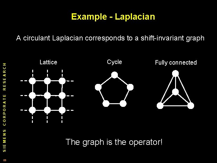
Example - Laplacian Lattice Cycle Fully connected SIEMENS CORPORATE RESEARCH A circulant Laplacian corresponds to a shift invariant graph 59 The graph is the operator!

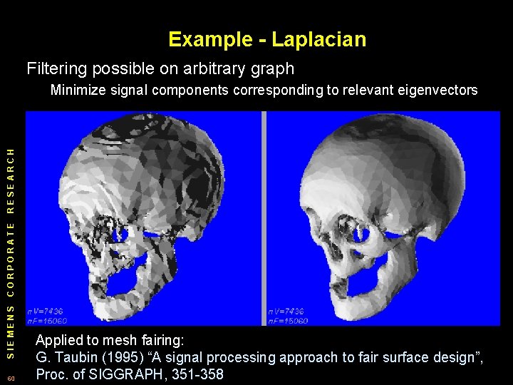
Example - Laplacian Filtering possible on arbitrary graph SIEMENS CORPORATE RESEARCH Minimize signal components corresponding to relevant eigenvectors 60 Applied to mesh fairing: G. Taubin (1995) “A signal processing approach to fair surface design”, Proc. of SIGGRAPH, 351 358

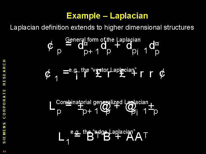
Example – Laplacian definition extends to higher dimensional structures General form of the Laplacian SIEMENS CORPORATE RESEARCH ¤ ¤ ¢ p = dp+ d d p¡ 1 p 61 ¢ 1 = ¡ r £ +r r ¢ e. g. , the “vector Laplacian” L p = ±p+ 1 @p + @p¡ 1 ±p Combinatorial generalized Laplacian e. g. , the “edge Laplacian” L 1 = B T B + AA T

Outline 0) Introduction 1) Theory – Combinatorial and continuous space SIEMENS CORPORATE RESEARCH a) Ingredients of continuous calculus 62 b) Ingredients of combinatorial calculus c) Example 1: Stokes Theorem d) Example 2: Helmholtz decomposition e) Example 3: Laplacian 2) Practice – Segmentation a) Reformulation of the Mumford Shah i) Formulation ii) Results b) Random walker algorithm i) Principle ii) Formulation iii) Results 3) Conclusion

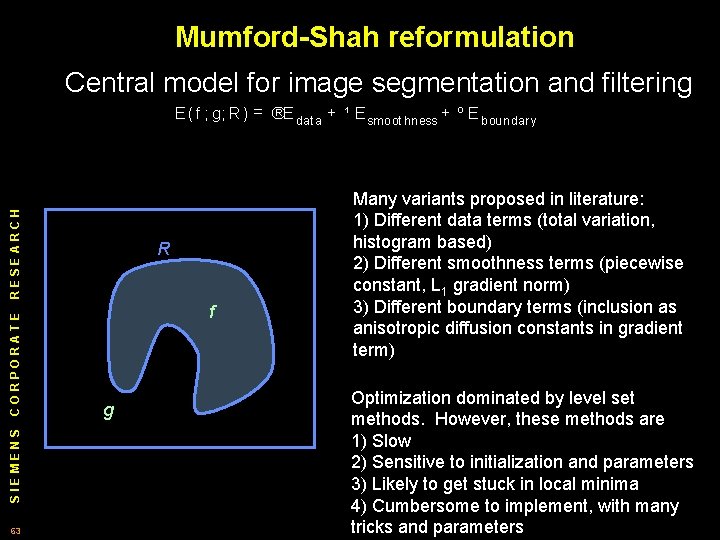
Mumford-Shah reformulation Central model for image segmentation and filtering SIEMENS CORPORATE RESEARCH E (f ; g; R) = ®E dat a + ¹ E sm oot hness + º E b oundar y 63 R f g Many variants proposed in literature: 1) Different data terms (total variation, histogram based) 2) Different smoothness terms (piecewise constant, L 1 gradient norm) 3) Different boundary terms (inclusion as anisotropic diffusion constants in gradient term) Optimization dominated by level set methods. However, these methods are 1) Slow 2) Sensitive to initialization and parameters 3) Likely to get stuck in local minima 4) Cumbersome to implement, with many tricks and parameters

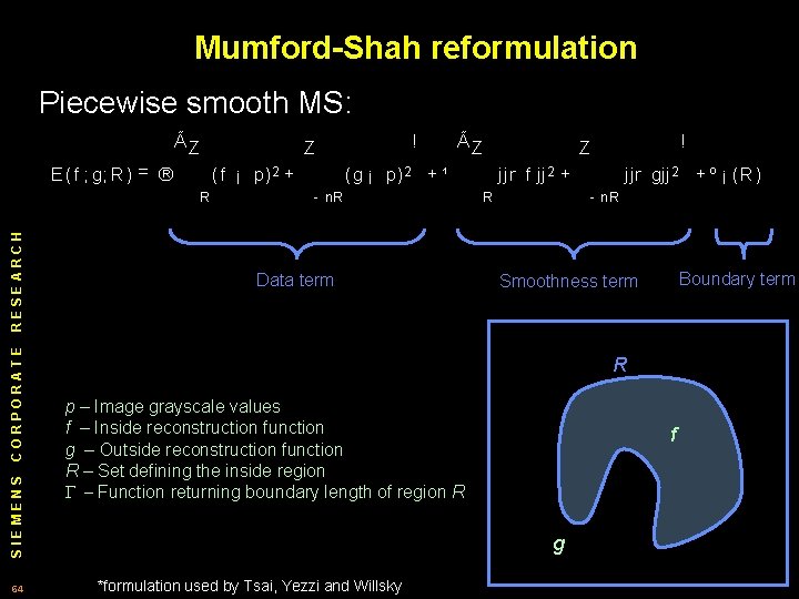
Mumford-Shah reformulation Piecewise smooth MS: ÃZ E (f ; g; R) = ® (f ¡ p) 2 + SIEMENS CORPORATE RESEARCH R 64 ! Z ÃZ (g ¡ p) 2 + ¹ n. R Data term ! Z jjr f jj 2 + R jjr gjj 2 + º ¡ (R) n. R Boundary term Smoothness term R p – Image grayscale values f – Inside reconstruction function g – Outside reconstruction function R – Set defining the inside region Г – Function returning boundary length of region R f g *formulation used by Tsai, Yezzi and Willsky

Mumford-Shah reformulation Data term Z SIEMENS CORPORATE RESEARCH E 1 (f ; g; R) = 65 Z (f ¡ p) 2 + R (g ¡ p) 2 n. R Question: What geometric structure to associate variables with? Answer: Image intensities a scalar field, should be associated with nodes If p is a node quantity, then f and g must be node quantities and R must be a set of nodes Therefore, we have the reformulation E 1 (f ; g; R) = r T (f ¡ p) 2 + (1 ¡ r ) T (g ¡ p) 2 r is a chain represented as an indicator vector, i. e. , ( ri = 1 if vi 2 R; 0 ot herwise:

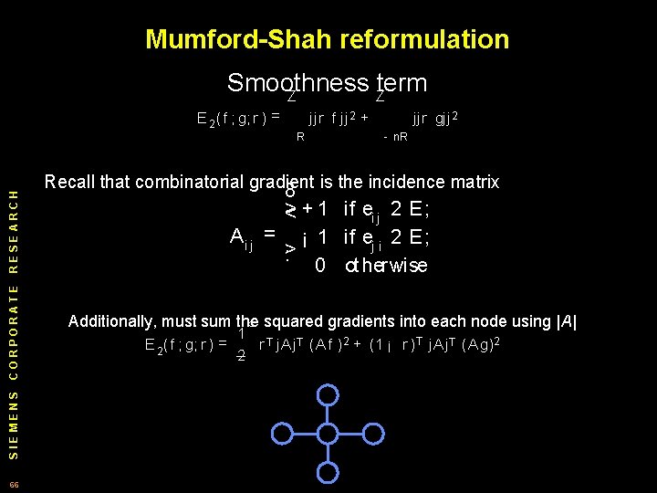
Mumford-Shah reformulation Smoothness term Z Z SIEMENS CORPORATE RESEARCH E 2 (f ; g; r ) = 66 jjr f jj 2 + R jjr gjj 2 n. R Recall that combinatorial gradient 8 is the incidence matrix Ai j > < + 1 if ei j 2 E ; = ¡ 1 if e 2 E ; ji > : 0 ot herwise Additionally, must sum the ³ squared gradients into each node´ using |A| E 2 (f ; g; r ) = 1 T r j. Aj T (Af ) 2 + (1 ¡ r ) T j. Aj T (Ag) 2 2

Mumford-Shah reformulation Boundary term E 3 (f ; g; r ) = ¡ (R) SIEMENS CORPORATE RESEARCH The boundary of a group of nodes is the set of edges exiting the group 67 This quantity is calculated via the boundary operator (incidence matrix) E 3 (f ; g; r ) = 1 T j. A T r j

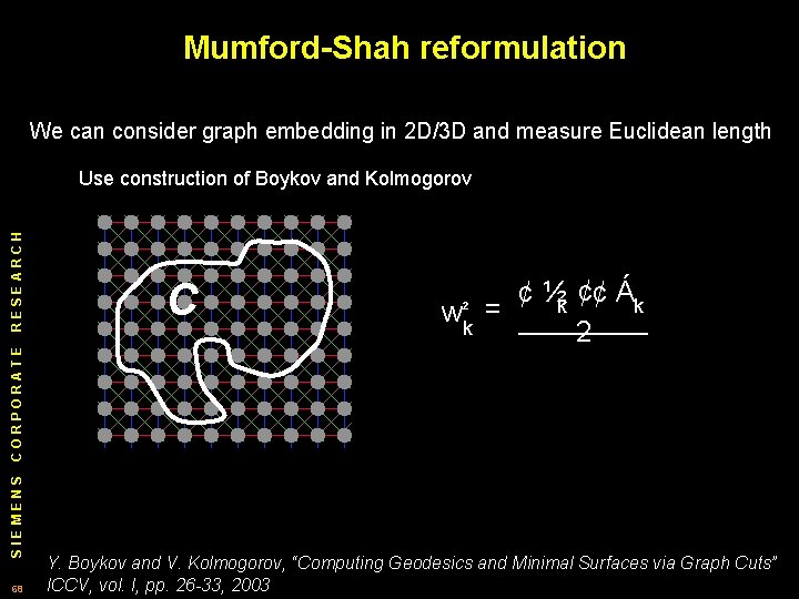
Mumford-Shah reformulation We can consider graph embedding in 2 D/3 D and measure Euclidean length SIEMENS CORPORATE RESEARCH Use construction of Boykov and Kolmogorov 68 C ¢¢ Ák ½ ¢ k wk² = 2 Y. Boykov and V. Kolmogorov, “Computing Geodesics and Minimal Surfaces via Graph Cuts” ICCV, vol. I, pp. 26 -33, 2003

Mumford-Shah reformulation Final form ÃZ E (f ; g; R) = ® (f ¡ p) 2 + SIEMENS CORPORATE RESEARCH R 69 Continuous ! ÃZ Z ³ (g ¡ p) 2 + ¹ n. R Z jjr f jj 2 + R Combinatorial ´ ³ E (f ; g; R) = ® r T (f ¡ p) 2 + (1 ¡ r ) T (g ¡ p) 2 + jjr gjj 2 + º ¡ (R) n. R ´ 1 T T 2 2 T T r j. A j (A f ) + (1 ¡ r ) j. Aj (A g) + 1 T j. A r j 2 Looks intimidating, but 1) 2) 2) ! Represents, in matrix vector form, the operations used to actually calculate energy Easy to optimize

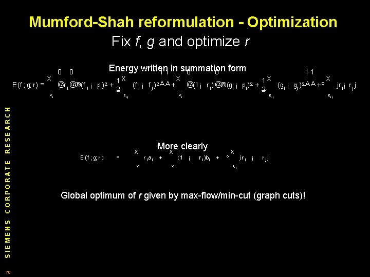
Mumford-Shah reformulation - Optimization Fix f, g and optimize r E (f ; g; r ) = X 0 Energy written 1 1 in summation 0 0 form 0 @r @®(f ¡ p ) 2 + i i i 2 SIEMENS CORPORATE RESEARCH vi 1 X 70 E (f ; g; r ) = (f i ¡ f j ) 2 A A + ei j X @(1 ¡ r ) @®(g ¡ p ) 2 + i i i vi X vi r i ai More clearly X (1 ¡ + vi r i )bi + º X jr i ¡ 1 X 2 11 (gi ¡ gj ) 2 A A + º ei j rj j ei j Global optimum of r given by max flow/min cut (graph cuts)! X ei j jr i ¡ r j j

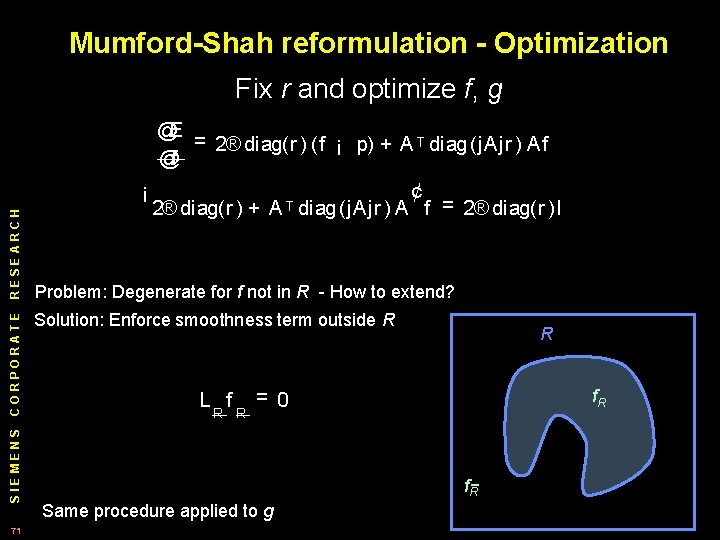
Mumford-Shah reformulation - Optimization Fix r and optimize f, g @E = 2® diag(r ) (f ¡ p) + A T diag (j. Ajr ) Af @f SIEMENS CORPORATE RESEARCH ¡ 71 2® diag(r ) + AT ¢ diag (j. Ajr ) A f = 2® diag(r )I Problem: Degenerate for f not in R How to extend? Solution: Enforce smoothness term outside R L f R R R = 0 f. R Same procedure applied to g

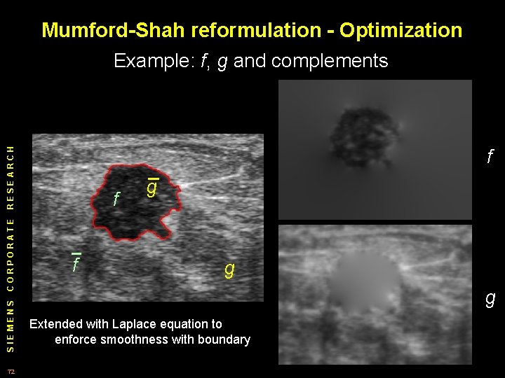
Mumford-Shah reformulation - Optimization Example: f, g and complements SIEMENS CORPORATE RESEARCH f 72 f f g g g Extended with Laplace equation to enforce smoothness with boundary

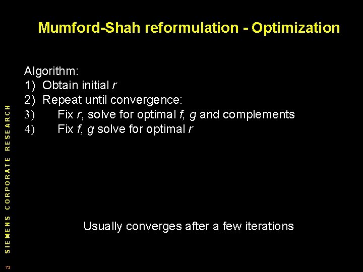
Algorithm: 1) Obtain initial r 2) Repeat until convergence: 3) Fix r, solve for optimal f, g and complements 4) Fix f, g solve for optimal r SIEMENS CORPORATE RESEARCH Mumford-Shah reformulation - Optimization 73 Usually converges after a few iterations

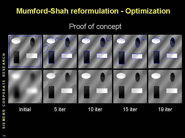
Mumford-Shah reformulation - Optimization SIEMENS CORPORATE RESEARCH Proof of concept 74 Initial 5 iter 10 iter 15 iter 19 iter

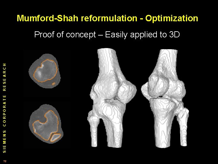
Mumford-Shah reformulation - Optimization SIEMENS CORPORATE RESEARCH Proof of concept – Easily applied to 3 D 75

Outline 0) Introduction 1) Theory – Combinatorial and continuous space SIEMENS CORPORATE RESEARCH a) Ingredients of continuous calculus 76 b) Ingredients of combinatorial calculus c) Example 1: Stokes Theorem d) Example 2: Helmholtz decomposition e) Example 3: Laplacian 2) Practice – Segmentation a) Reformulation of the Mumford Shah i) Formulation ii) Results b) Random walker algorithm i) Principle ii) Formulation iii) Results 3) Conclusion

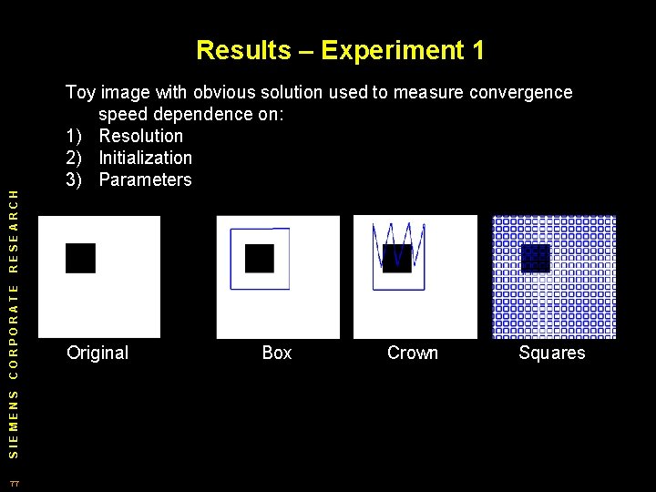
SIEMENS CORPORATE RESEARCH Results – Experiment 1 77 Toy image with obvious solution used to measure convergence speed dependence on: 1) Resolution 2) Initialization 3) Parameters Original Box Crown Squares

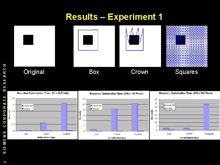
SIEMENS CORPORATE RESEARCH Results – Experiment 1 78 Original Box Crown Squares

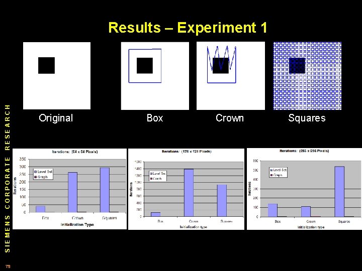
SIEMENS CORPORATE RESEARCH Results – Experiment 1 79 Original Box Crown Squares

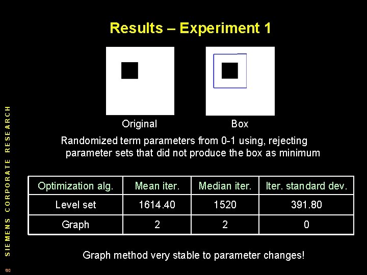
SIEMENS CORPORATE RESEARCH Results – Experiment 1 80 Original Box Randomized term parameters from 0 1 using, rejecting parameter sets that did not produce the box as minimum Optimization alg. Mean iter. Median iter. Iter. standard dev. Level set 1614. 40 1520 391. 80 Graph 2 2 0 Graph method very stable to parameter changes!

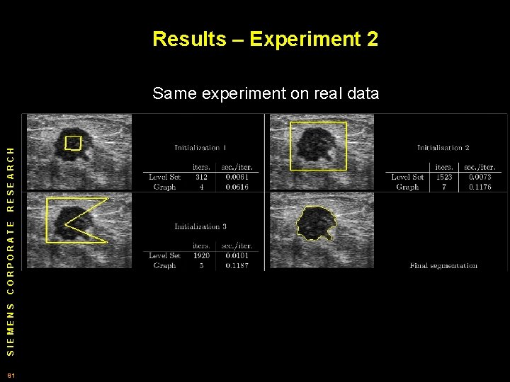
Results – Experiment 2 SIEMENS CORPORATE RESEARCH Same experiment on real data 81

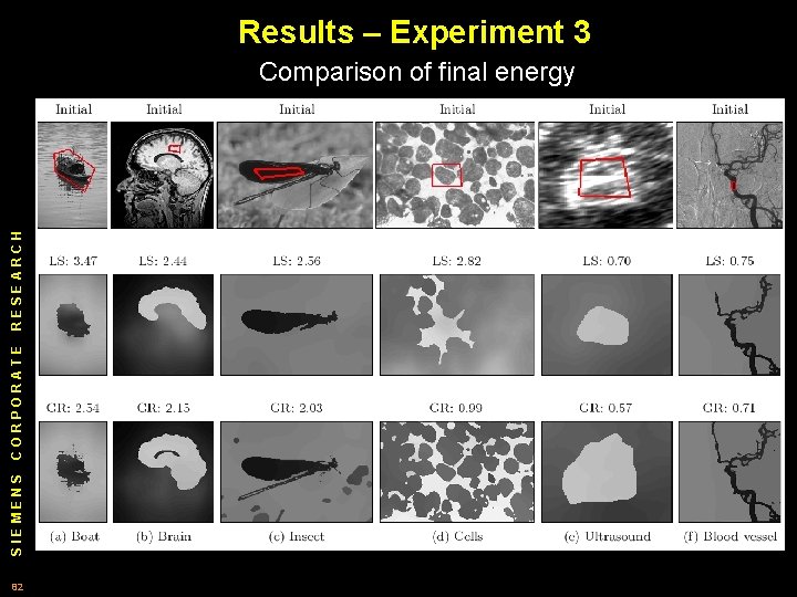
Results – Experiment 3 SIEMENS CORPORATE RESEARCH Comparison of final energy 82

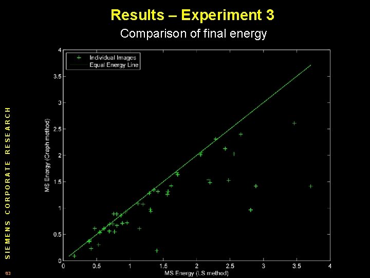
Results – Experiment 3 SIEMENS CORPORATE RESEARCH Comparison of final energy 83

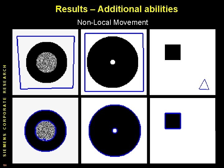
Results – Additional abilities SIEMENS CORPORATE RESEARCH Non Local Movement 84

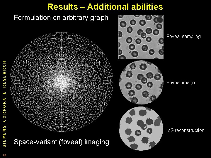
Results – Additional abilities Formulation on arbitrary graph RESEARCH Foveal sampling SIEMENS CORPORATE Foveal image 85 MS reconstruction Space variant (foveal) imaging

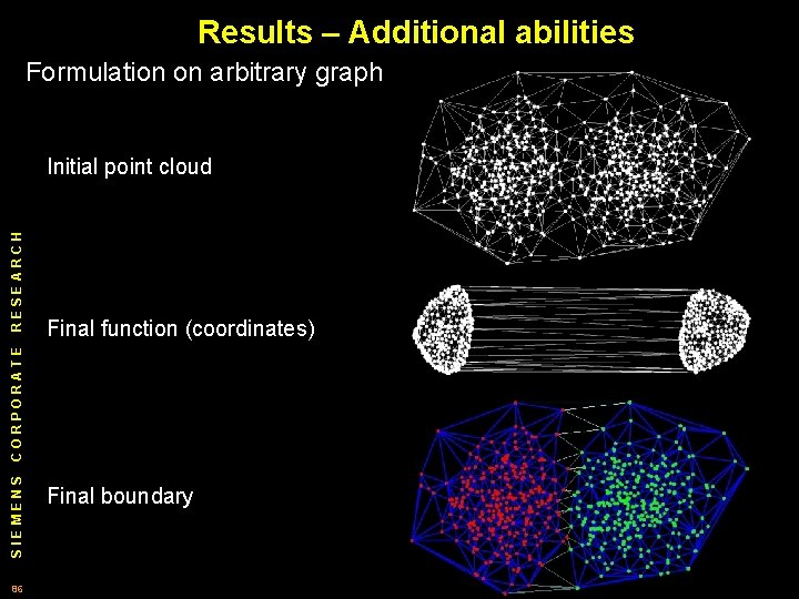
Results – Additional abilities Formulation on arbitrary graph Final function (coordinates) SIEMENS CORPORATE RESEARCH Initial point cloud 86 Final boundary

Outline 0) Introduction 1) Theory – Combinatorial and continuous space SIEMENS CORPORATE RESEARCH a) Ingredients of continuous calculus 87 b) Ingredients of combinatorial calculus c) Example 1: Stokes Theorem d) Example 2: Helmholtz decomposition e) Example 3: Laplacian 2) Practice – Segmentation a) Reformulation of the Mumford Shah i) Formulation ii) Results b) Random walker algorithm i) Principle ii) Formulation iii) Results 3) Conclusion

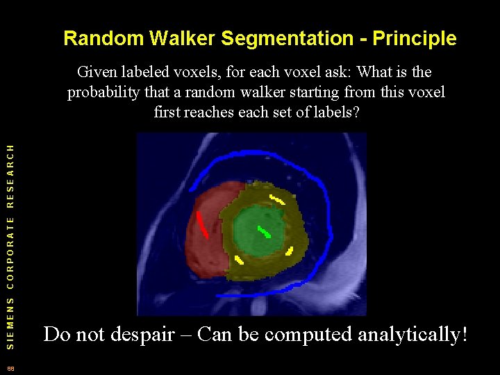
Random Walker Segmentation - Principle SIEMENS CORPORATE RESEARCH Given labeled voxels, for each voxel ask: What is the probability that a random walker starting from this voxel first reaches each set of labels? 88 Do not despair – Can be computed analytically!

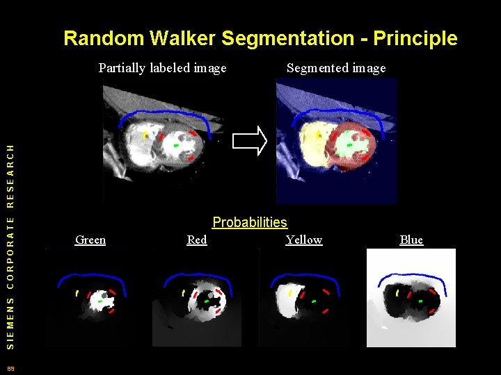
Random Walker Segmentation - Principle Segmented image SIEMENS CORPORATE RESEARCH Partially labeled image 89 Probabilities Green Red Yellow Blue

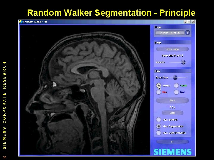
SIEMENS CORPORATE RESEARCH Random Walker Segmentation - Principle 90

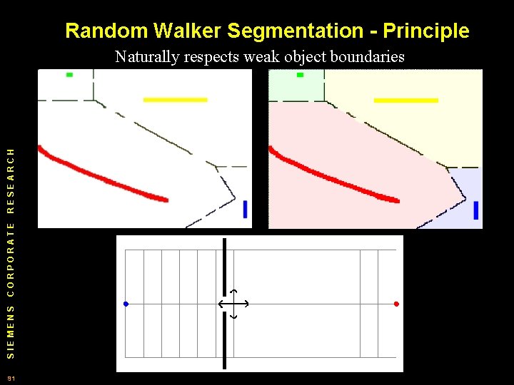
Random Walker Segmentation - Principle SIEMENS CORPORATE RESEARCH Naturally respects weak object boundaries 91

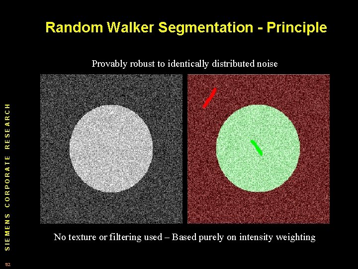
Random Walker Segmentation - Principle SIEMENS CORPORATE RESEARCH Provably robust to identically distributed noise 92 No texture or filtering used – Based purely on intensity weighting

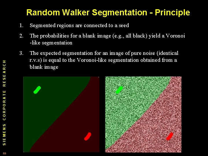
SIEMENS CORPORATE RESEARCH Random Walker Segmentation - Principle 93 1. Segmented regions are connected to a seed 2. The probabilities for a blank image (e. g. , all black) yield a Voronoi -like segmentation 3. The expected segmentation for an image of pure noise (identical r. v. s) is equal to the Voronoi-like segmentation obtained from a blank image

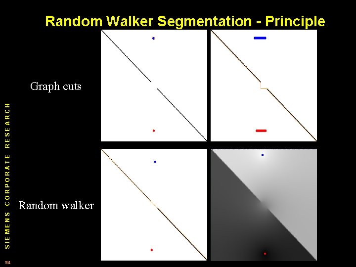
Random Walker Segmentation - Principle SIEMENS CORPORATE RESEARCH Graph cuts 94 Random walker

SIEMENS CORPORATE RESEARCH Random Walker Segmentation - Principle 95

Outline 0) Introduction 1) Theory – Combinatorial and continuous space SIEMENS CORPORATE RESEARCH a) Ingredients of continuous calculus 96 b) Ingredients of combinatorial calculus c) Example 1: Stokes Theorem d) Example 2: Helmholtz decomposition e) Example 3: Laplacian 2) Practice – Segmentation a) Reformulation of the Mumford Shah i) Formulation ii) Results b) Random walker algorithm i) Principle ii) Formulation iii) Results 3) Conclusion

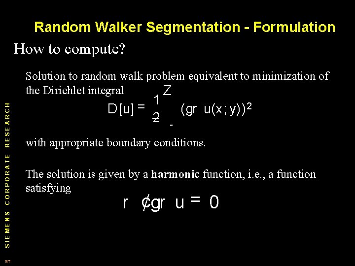
Random Walker Segmentation - Formulation How to compute? SIEMENS CORPORATE RESEARCH Solution to random walk problem equivalent to minimization of the Dirichlet integral Z 97 1 D [u] = 2 (gr u(x; y)) 2 with appropriate boundary conditions. The solution is given by a harmonic function, i. e. , a function satisfying r ¢gr u = 0

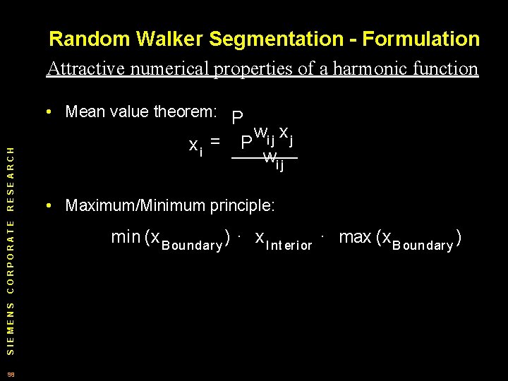
Random Walker Segmentation - Formulation Attractive numerical properties of a harmonic function SIEMENS CORPORATE RESEARCH • Mean value theorem: P 98 xi = wi j x j P wi j • Maximum/Minimum principle: min (x B oundar y ) · x I nt er i or · max (x B oundar y )

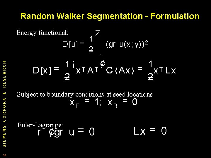
Random Walker Segmentation - Formulation Energy functional: SIEMENS CORPORATE RESEARCH 1 D [u] = 2 99 Z (gr u(x; y)) 2 1¡ T T¢ 1 T D [x] = x A C (Ax) = x L x 2 2 Subject to boundary conditions at seed locations x F = 1; x B = 0 Euler-Lagrange: r ¢gr u = 0 Lx = 0

Random Walker Segmentation - Formulation SIEMENS CORPORATE RESEARCH Algorithm summary: 100 1. Generate weights based on image intensities 2. Build Laplacian matrix 3. Solve system of equations for each label 4. Assign pixel (voxel) to label for which it has the highest probability

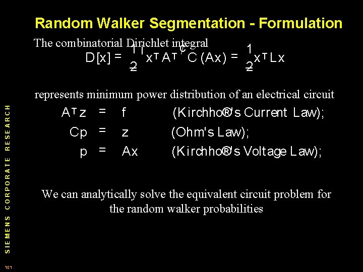
Random Walker Segmentation - Formulation The combinatorial Dirichlet integral ¡ ¢ D [x] = 1 T T 1 T = x A C (Ax) x Lx 2 2 SIEMENS CORPORATE RESEARCH represents minimum power distribution of an electrical circuit 101 AT z = Cp = f z Ax (K irchho®'s Current Law); (Ohm's Law); (K irchho®'s Volt age Law); We can analytically solve the equivalent circuit problem for the random walker probabilities

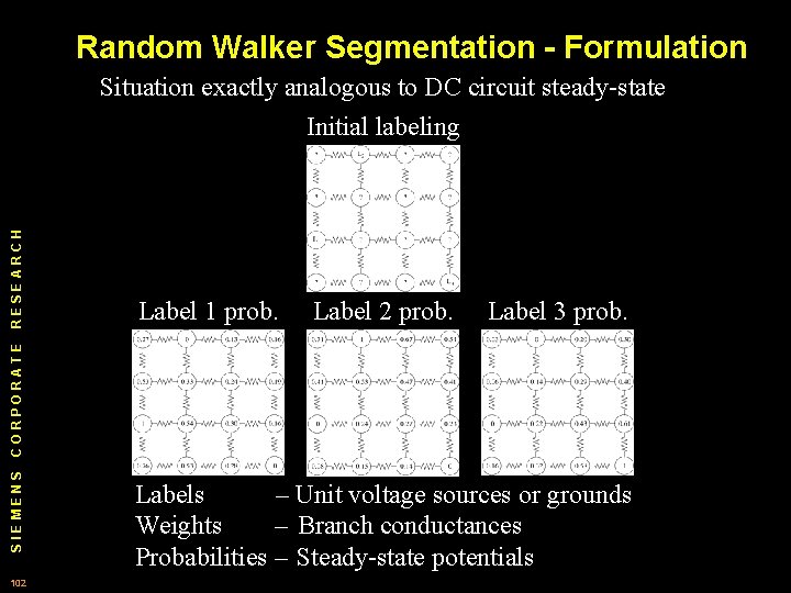
Random Walker Segmentation - Formulation Label 1 prob. Label 2 prob. Label 3 prob. SIEMENS CORPORATE RESEARCH Situation exactly analogous to DC circuit steady-state Initial labeling 102 Labels – Unit voltage sources or grounds Weights – Branch conductances Probabilities – Steady-state potentials

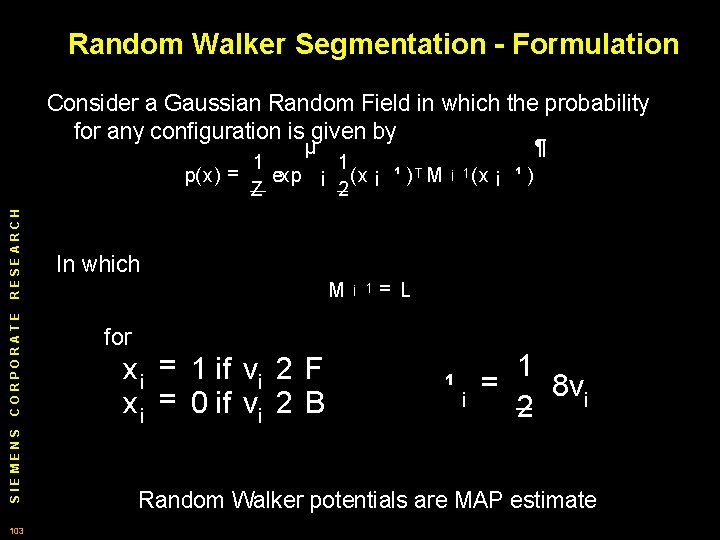
Random Walker Segmentation - Formulation Consider a Gaussian Random Field in which the probability for any configuration is given by µ SIEMENS CORPORATE RESEARCH p(x) = 103 1 1 exp ¡ (x ¡ ¹ ) T M 2 Z In which M for x i = 1 if vi 2 F x i = 0 if vi 2 B ¡ 1 ¶ ¡ 1 (x ¡ ¹) = L 1 8 vi ¹i = 2 Random Walker potentials are MAP estimate

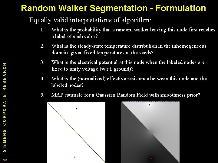
Random Walker Segmentation - Formulation SIEMENS CORPORATE RESEARCH Equally valid interpretations of algorithm: 104 1. What is the probability that a random walker leaving this node first reaches a label of each color? 2. What is the steady-state temperature distribution in the inhomogeneous domain, given fixed temperatures at the seeds? 3. What is the electrical potential at this node when the labeled nodes are fixed to unity voltage (w. r. t. ground)? 4. What is the (normalized) effective resistance between this node and the labeled nodes? 5. MAP estimate for a Gaussian Random Field with smoothness prior?

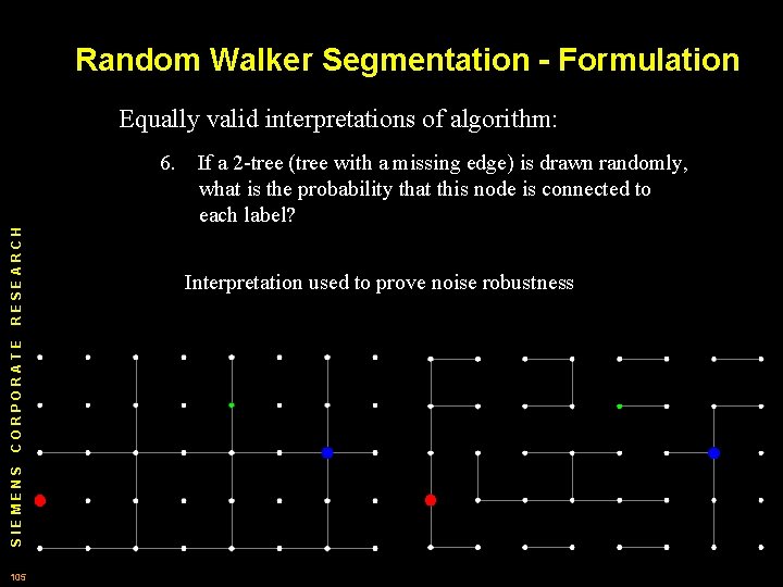
Random Walker Segmentation - Formulation Equally valid interpretations of algorithm: SIEMENS CORPORATE RESEARCH 6. 105 If a 2 -tree (tree with a missing edge) is drawn randomly, what is the probability that this node is connected to each label? Interpretation used to prove noise robustness

Random Walker Segmentation - Formulation ‘Algorithm A’ G i ven Foreground F and Background B Seeds, q 2 R+ h. P i 1 L et x à arg min k. C 12 Axkq = (wi j jx i ¡ x j j) q q , SIEMENS CORPORATE RESEARCH q 106 ei j 2 E subject t o x(F ) = 1 and x(B() = 0. 1 if x i ¸ Out put Segment at ion si = 0 if x i < Choice of q determines solution properties: q=1 Graph Cuts q=2 Random Walker q=∞ Shortest Paths 1; 2 1: 2 Continuous Z equivalent L et u à arg min kgr ukqq subject t o u (F ) = 1 and u (B ) = 0:

Outline 0) Introduction 1) Theory – Combinatorial and continuous space SIEMENS CORPORATE RESEARCH a) Ingredients of continuous calculus 107 b) Ingredients of combinatorial calculus c) Example 1: Stokes Theorem d) Example 2: Helmholtz decomposition e) Example 3: Laplacian 2) Practice – Segmentation a) Reformulation of the Mumford Shah i) Formulation ii) Results b) Random walker algorithm i) Principle ii) Formulation iii) Results 3) Conclusion

SIEMENS CORPORATE RESEARCH Random Walker Segmentation - Results 108

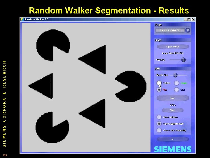
SIEMENS CORPORATE RESEARCH Random Walker Segmentation - Results 109

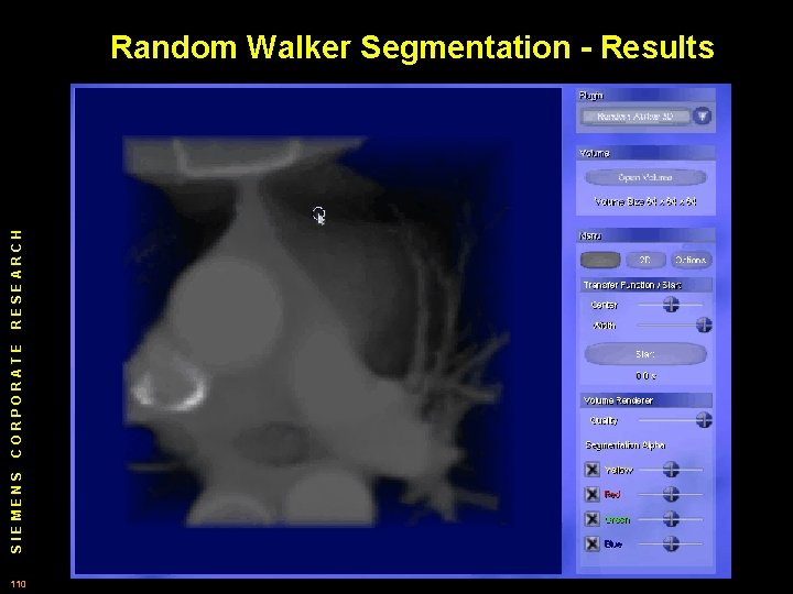
SIEMENS CORPORATE RESEARCH Random Walker Segmentation - Results 110

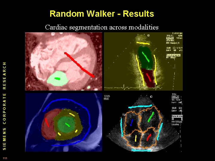
Random Walker - Results SIEMENS CORPORATE RESEARCH Cardiac segmentation across modalities 111

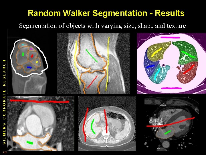
Random Walker Segmentation - Results SIEMENS CORPORATE RESEARCH Segmentation of objects with varying size, shape and texture 112

Outline 0) Introduction 1) Theory – Combinatorial and continuous space SIEMENS CORPORATE RESEARCH a) Ingredients of continuous calculus 113 b) Ingredients of combinatorial calculus c) Example 1: Stokes Theorem d) Example 2: Helmholtz decomposition e) Example 3: Laplacian 2) Practice – Segmentation a) Reformulation of the Mumford Shah i) Formulation ii) Results b) Random walker algorithm i) Principle ii) Formulation iii) Results 3) Conclusion

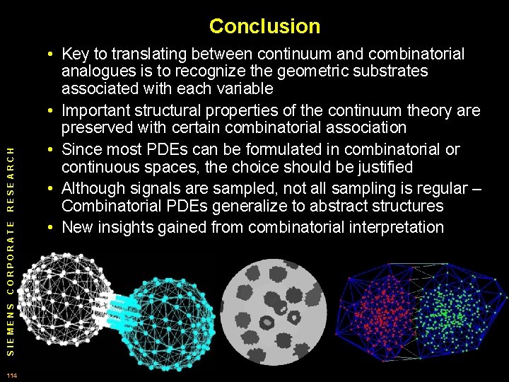
SIEMENS CORPORATE RESEARCH Conclusion 114 • Key to translating between continuum and combinatorial analogues is to recognize the geometric substrates associated with each variable • Important structural properties of the continuum theory are preserved with certain combinatorial association • Since most PDEs can be formulated in combinatorial or continuous spaces, the choice should be justified • Although signals are sampled, not all sampling is regular – Combinatorial PDEs generalize to abstract structures • New insights gained from combinatorial interpretation

More information: Conclusion Recommended reading Books: SIEMENS CORPORATE RESEARCH 1) Strang, G. (1986), “Introduction to Applied Mathematics”, Wellesley-Cambridge Press 2) Frankel, T. (2003), “The Geometry of Physics”, 2 nd ed. , Cambridge University Press 3) Burke, W. (2003), “Applied Differential Geometry”, Cambridge University Press Papers: 1) Branin Jr, F. (1966), “The Algebraic-Topological Basis for Network Analogies and for Vector Calculus”, Symposium on Generalized Networks, 453 -491 2) Tonti, E. (1976), “The Reason for Analogies between Physical Theories”, in Applied Mathematical Modeling, Vol 1, 37 -50 3) Mattiussi, C. (2000), “The Finite Volume, Finite Difference, and Finite Elements Methods as Numerical Methods for Physical Field Problems”, Advances in Imaging and Electron Physics, 1 -146 My work Webpage: http: //cns. bu. edu/~lgrady Random walker segmentation demo page: http: //cns. bu. edu/~lgrady/random_walker_demo. html MATLAB toolbox for combinatorial image processing at: http: //eslab. bu. edu/software/graphanalysis/ 115