Reproducing Graphs Chris Cannings Richard Southwell Gene Networks

Reproducing Graphs Chris Cannings & Richard Southwell

Gene Networks

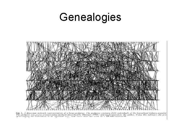
Genealogies

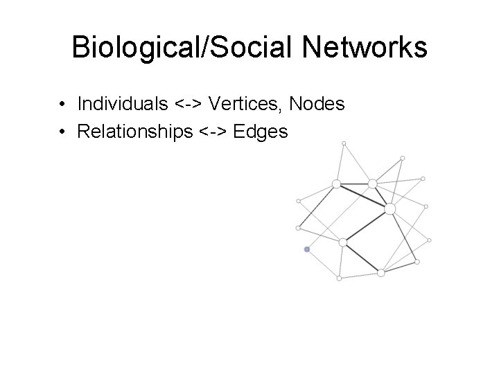
Biological/Social Networks • Individuals <-> Vertices, Nodes • Relationships <-> Edges

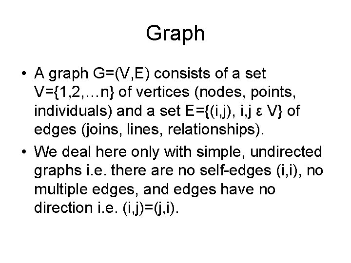
Graph • A graph G=(V, E) consists of a set V={1, 2, …n} of vertices (nodes, points, individuals) and a set E={(i, j), i, j ε V} of edges (joins, lines, relationships). • We deal here only with simple, undirected graphs i. e. there are no self-edges (i, i), no multiple edges, and edges have no direction i. e. (i, j)=(j, i).

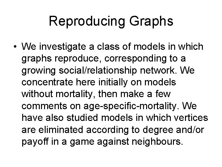
Reproducing Graphs • We investigate a class of models in which graphs reproduce, corresponding to a growing social/relationship network. We concentrate here initially on models without mortality, then make a few comments on age-specific-mortality. We have also studied models in which vertices are eliminated according to degree and/or payoff in a game against neighbours.

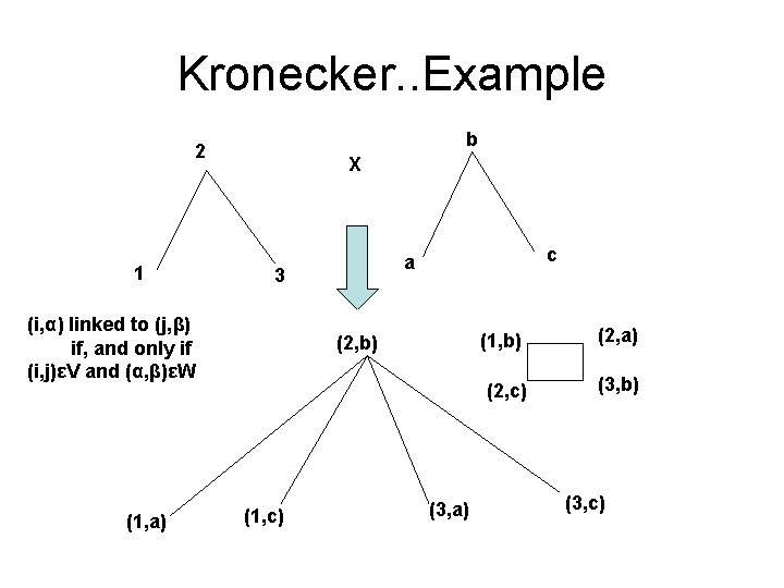
Graph Products • Given two graphs G 1=(V, E) and G 2=(W, F) then a graph product G 12 = G 1 X G 2 =(X, H) has X=V*W where * is the Cartesian product (i. e. X is the set of ordered pairs (v, w) where v ε V and w ε W). H depends on the particular product; there will be a rule which specifies which (v 1, w 1) and (v 2, w 2) join.

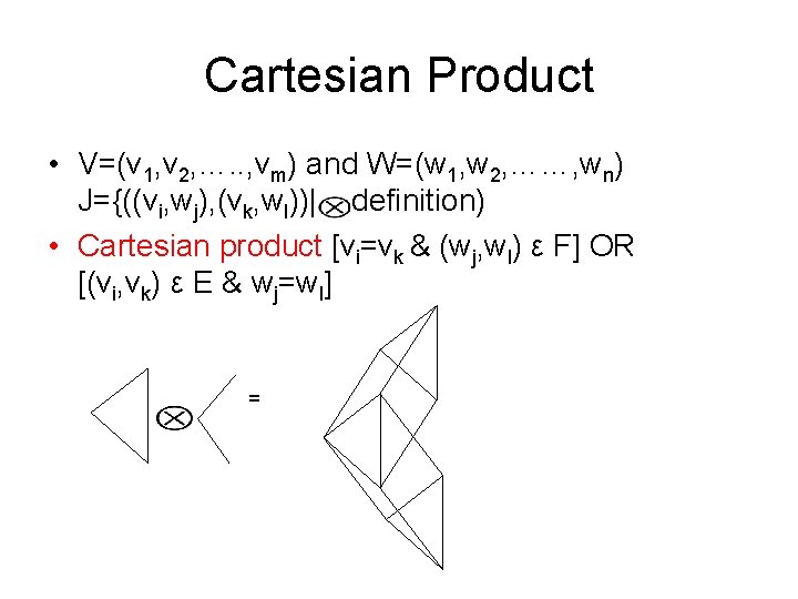
Cartesian Product • V=(v 1, v 2, …. . , vm) and W=(w 1, w 2, ……, wn) J={((vi, wj), (vk, wl))| definition) • Cartesian product [vi=vk & (wj, wl) ε F] OR [(vi, vk) ε E & wj=wl] =

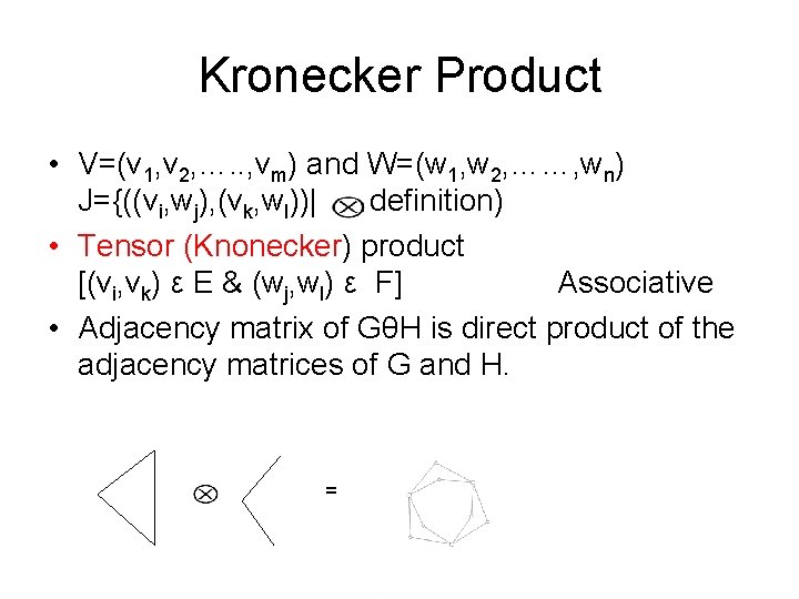
Kronecker Product • V=(v 1, v 2, …. . , vm) and W=(w 1, w 2, ……, wn) J={((vi, wj), (vk, wl))| definition) • Tensor (Knonecker) product [(vi, vk) ε E & (wj, wl) ε F] Associative • Adjacency matrix of GθH is direct product of the adjacency matrices of G and H. =

Kronecker. . Example b 2 1 X 3 (i, α) linked to (j, β) if, and only if (i, j)εV and (α, β)εW (1, a) c a (2, b) (1, c) (3, a) (1, b) (2, a) (2, c) (3, b) (3, c)

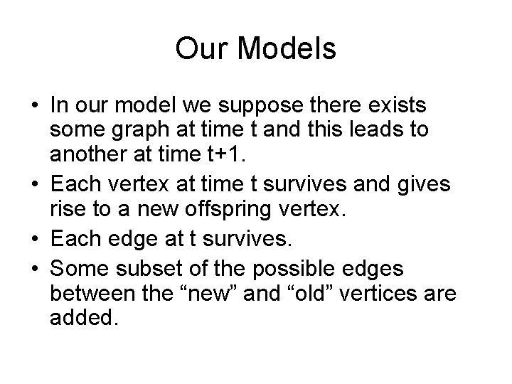
Our Models • In our model we suppose there exists some graph at time t and this leads to another at time t+1. • Each vertex at time t survives and gives rise to a new offspring vertex. • Each edge at t survives. • Some subset of the possible edges between the “new” and “old” vertices are added.

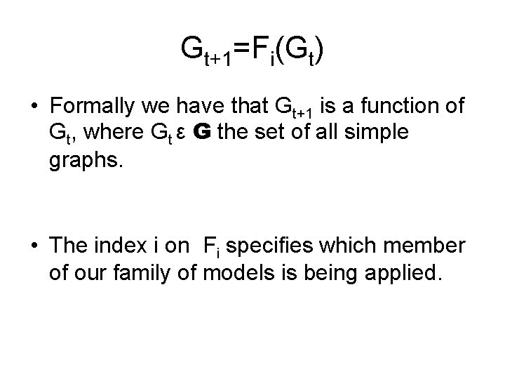
Gt+1=Fi(Gt) • Formally we have that Gt+1 is a function of Gt, where Gt ε G the set of all simple graphs. • The index i on Fi specifies which member of our family of models is being applied.

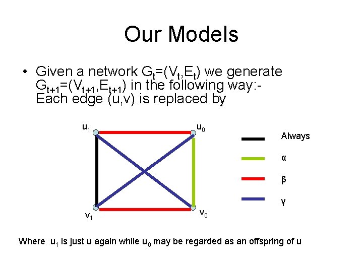
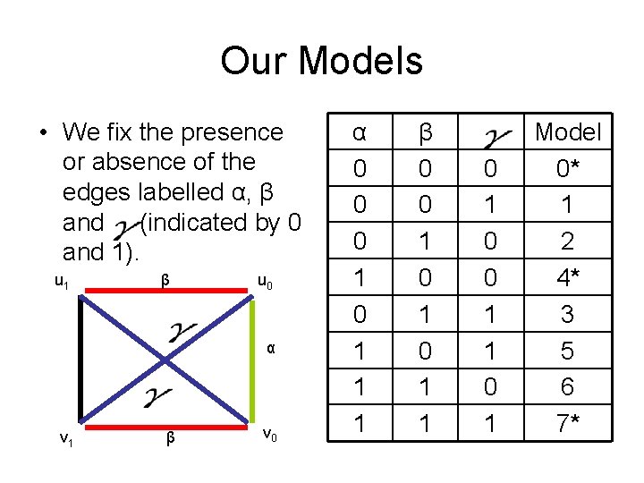
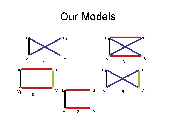
Our Models • Given a network Gt=(Vt, Et) we generate Gt+1=(Vt+1, Et+1) in the following way: Each edge (u, v) is replaced by u 1 u 0 Always α β γ v 1 v 0 Where u 1 is just u again while u 0 may be regarded as an offspring of u

Our Models • We fix the presence or absence of the edges labelled α, β and (indicated by 0 and 1). u 1 β u 0 α v 1 β v 0 α 0 0 0 1 1 1 β 0 0 1 0 1 1 0 1 Model 0* 1 2 4* 3 5 6 7*

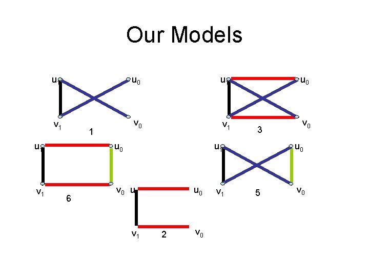
Our Models u 1 u 0 u 1 v 0 v 1 1 u 0 v 1 v 0 u 1 6 u 0 3 u 1 v 1 u 0 2 v 0 v 1 v 0 u 0 5 v 0

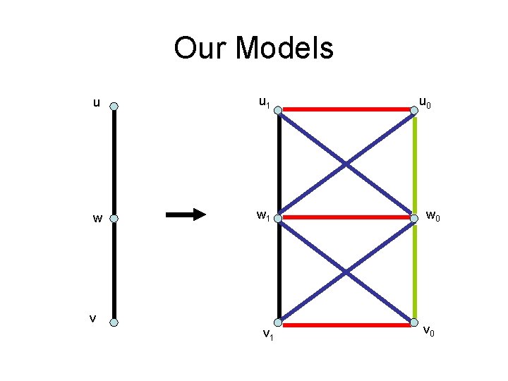
Our Models u u 1 w w 1 v v 1 u 0 w 0 v 0

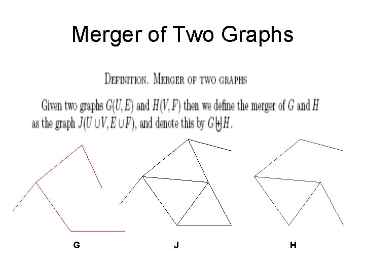
Merger of Two Graphs G J H

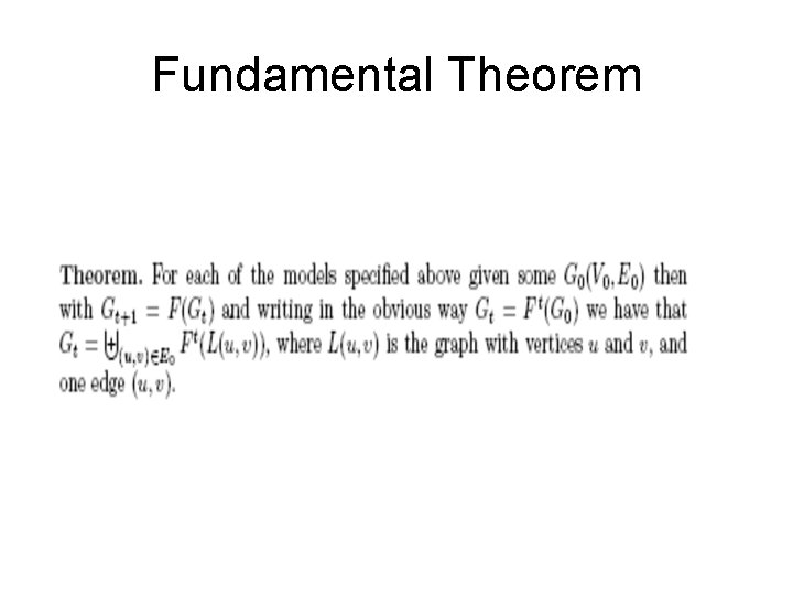
Fundamental Theorem

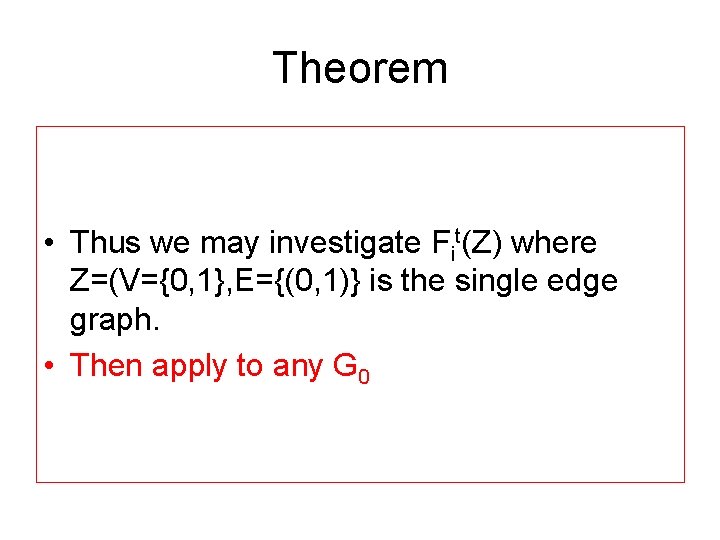
Theorem • Thus we may investigate Fit(Z) where Z=(V={0, 1}, E={(0, 1)} is the single edge graph. • Then apply to any G 0

Our Models u 1 u 0 u 1 v 0 v 1 1 u 0 v 1 v 0 u 1 6 u 0 3 u 1 v 1 u 0 2 v 0 v 1 v 0 u 0 5 v 0

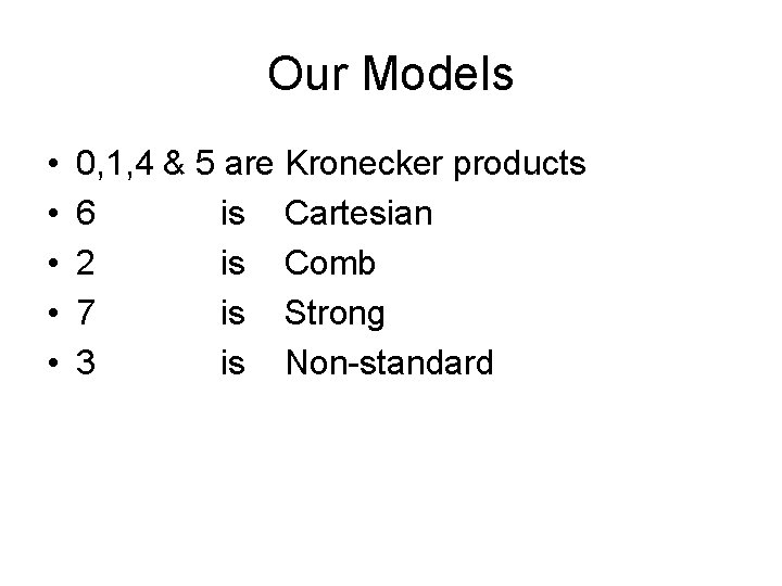
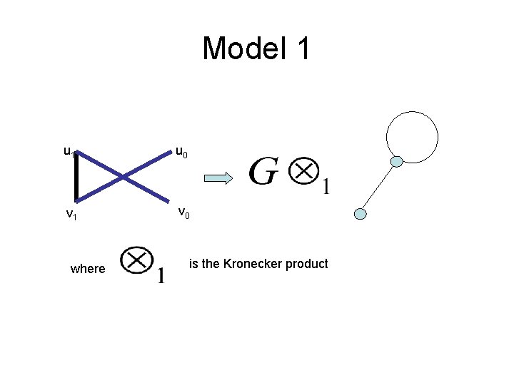
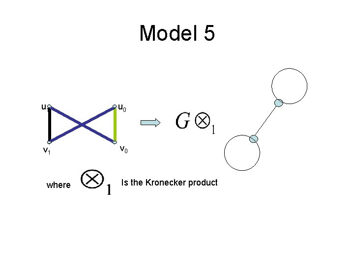
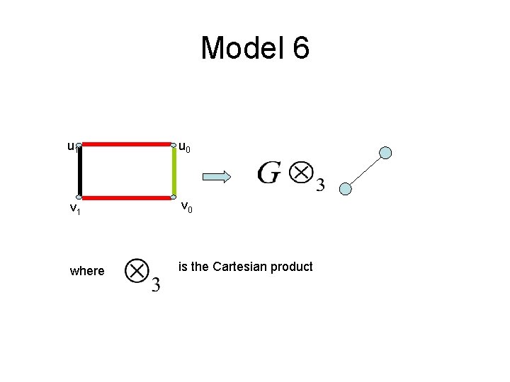
Our Models • • • 0, 1, 4 & 5 are Kronecker products 6 is Cartesian 2 is Comb 7 is Strong 3 is Non-standard

Model 1 u 0 v 1 v 0 where is the Kronecker product

Model 5 u 1 u 0 v 1 v 0 where Is the Kronecker product

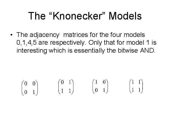
The “Knonecker” Models • Since the adjacency matrix of the Knonecker product of two graphs is the Knonecker product of the adjacency matrices we can exploit this for models 0, 1, 4 & 5

The “Knonecker” Models • The adjacency matrices for the four models 0, 1, 4, 5 are respectively. Only that for model 1 is interesting which is essentially the bitwise AND.

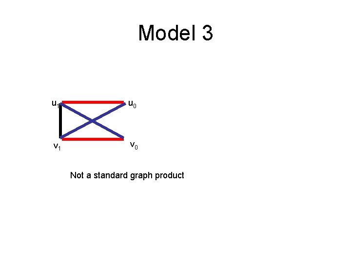
Model 3 u 1 u 0 v 1 v 0 Not a standard graph product

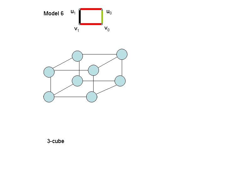
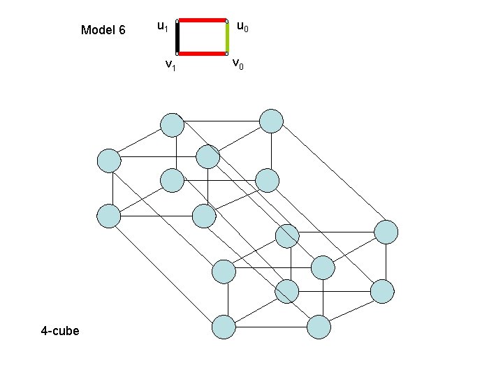
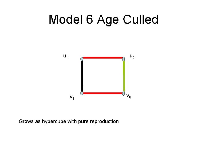
Model 6 u 1 u 0 v 1 v 0 where is the Cartesian product

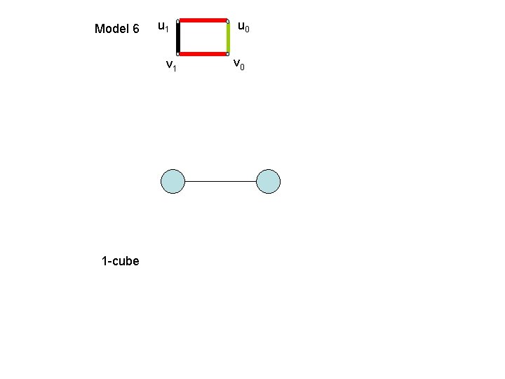
Model 6 u 1 v 1 1 -cube u 0 v 0

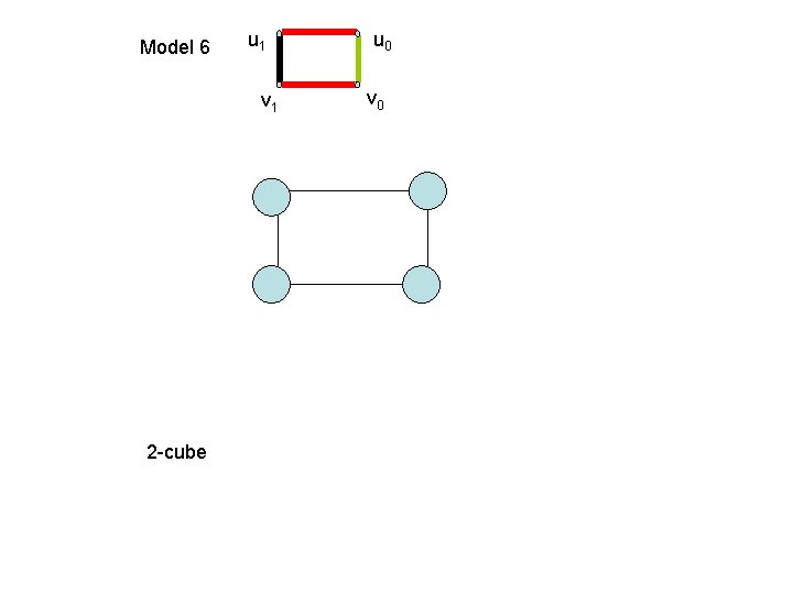
Model 6 u 1 v 1 2 -cube u 0 v 0

Model 6 u 1 v 1 3 -cube u 0 v 0

Model 6 u 1 v 1 4 -cube u 0 v 0

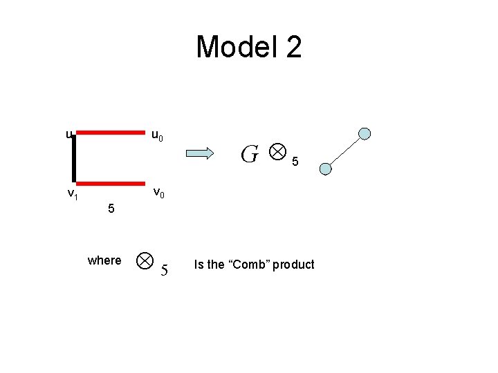
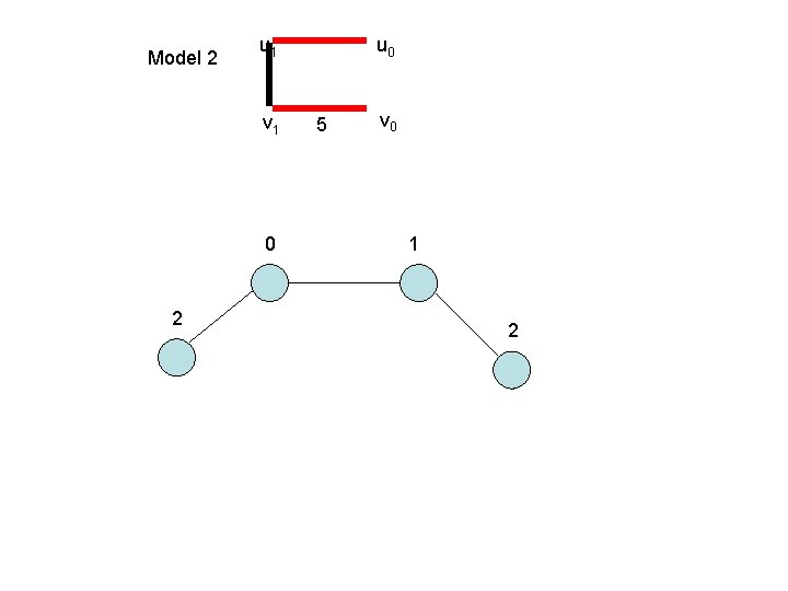
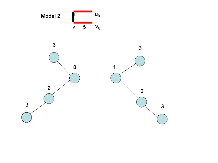
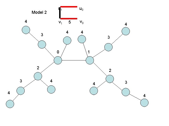
Model 2 u 1 u 0 v 1 v 0 G Ä5 5 where Ä5 Is the “Comb” product

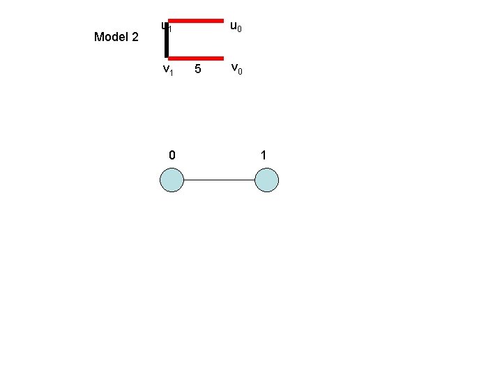
Model 2 u 1 v 1 0 u 0 5 v 0 1

Model 2 u 1 v 1 0 2 u 0 5 v 0 1 2

Model 2 u 1 v 1 u 0 5 v 0 3 3 0 2 3 1 2 3

u 1 Model 2 4 v 1 u 0 5 4 3 v 0 4 4 3 0 1 2 3 4 2 4 4 3 4

N. B…. . Binary Representation • If at time t we have a set of nodes {v 1, v 2, …. , vn} where each vi is a binary string then at time t+1 we have set of nodes {v 11, v 10, v 21, v 20, ……. . , vn 1, vn 0} where vi becomes vi 1 and is the parent of a new node vi 0. • All our models can be specified in terms of the nodes as binary strings and logical operations defining the edges.

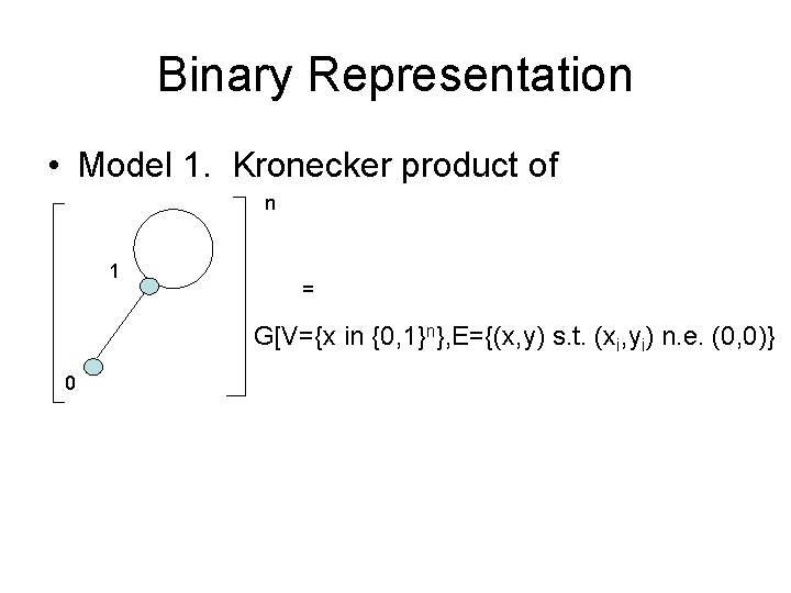
Binary Representation • Model 1. Kronecker product of n 1 = G[V={x in {0, 1}n}, E={(x, y) s. t. (xi, yi) n. e. (0, 0)} 0

Properties • 1. Chromatic Number • 2. Number of Vertices and Edges • 3. Distance Structure • 4. Degree Distribution • 5. Automorphism • 6. Generating all graphs as subgraphs.

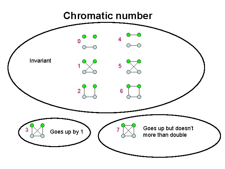
Chromatic number Invariant 0 4 1 5 2 3 Goes up by 1 6 7 Goes up but doesn’t more than double

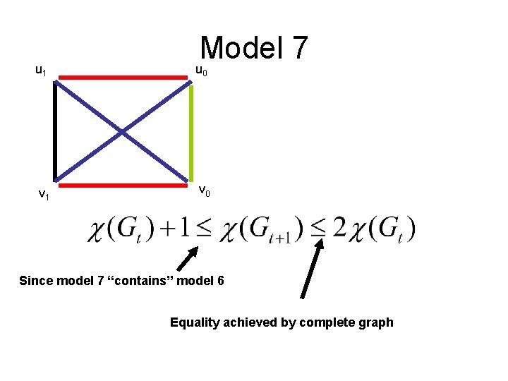
u 1 v 1 Model 7 u 0 v 0 Since model 7 “contains” model 6 Equality achieved by complete graph

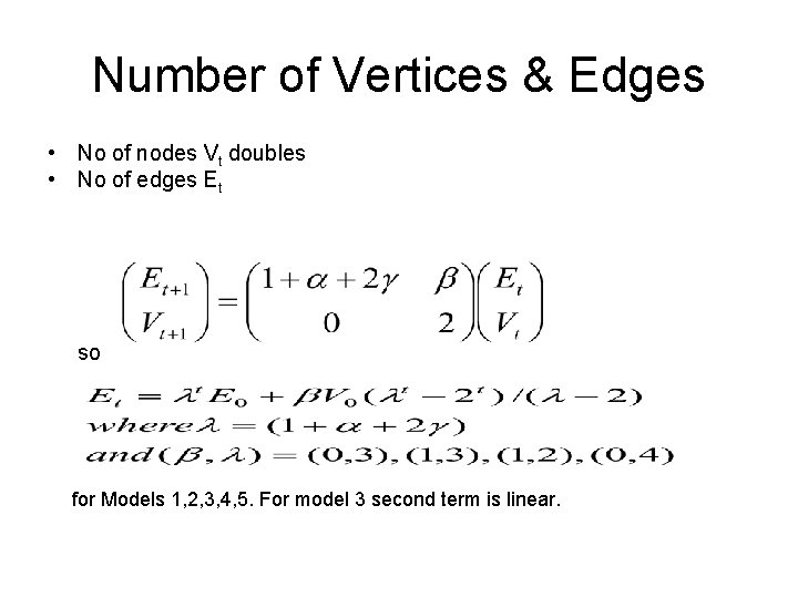
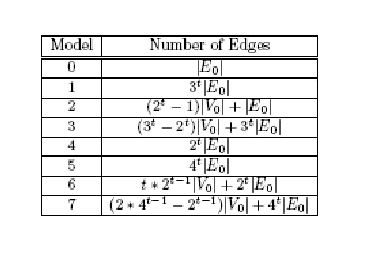
Number of Vertices & Edges • No of nodes Vt doubles • No of edges Et so for Models 1, 2, 3, 4, 5. For model 3 second term is linear.

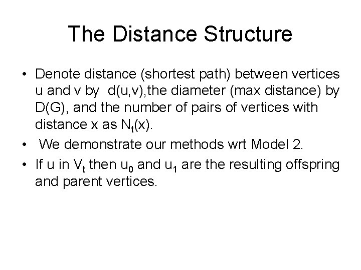
The Distance Structure • Denote distance (shortest path) between vertices u and v by d(u, v), the diameter (max distance) by D(G), and the number of pairs of vertices with distance x as Nt(x). • We demonstrate our methods wrt Model 2. • If u in Vt then u 0 and u 1 are the resulting offspring and parent vertices.

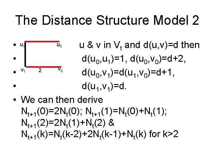
The Distance Structure Model 2 u • u u & v in Vt and d(u, v)=d then • d(u 0, u 1)=1, d(u 0, v 0)=d+2, v v 2 • d(u 0, v 1)=d(u 1, v 0)=d+1, • d(u 1, v 1)=d. • We can then derive Nt+1(0)=2 Nt(0); Nt+1(1)=Nt(0)+Nt(1); Nt+1(2)=2 Nt(1)+Nt(2) & Nt+1(k)=Nt(k-2)+2 Nt(k-1)+Nt(k) for k>2 1 0

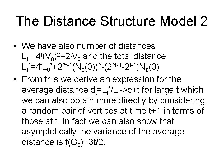
The Distance Structure Model 2 • We have also number of distances Lt =4 t(V 0)2+2 t. V 0 and the total distance Lt*=4 t. L 0*+22 t-1(N 0(0))2 -(22 t-1 -2 t-1)N 0(0) • From this we derive an expression for the average distance dt=Lt*/Lt->c+t for large t which we can also obtain more directly by considering a random pair of vertices at time t+1 in terms of those at t. In fact we can also show that asymptotically the variance of the average distance is f(G 0)+3 t/2.

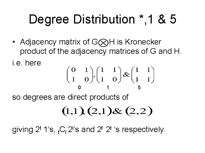
Degree Distribution *, 1 & 5 • Adjacency matrix of G H is Kronecker product of the adjacency matrices of G and H. i. e. here 0 1 5 so degrees are direct products of giving 2 t 1’s, t. Ci 2 i’s and 2 t 2 t ‘s respectively.

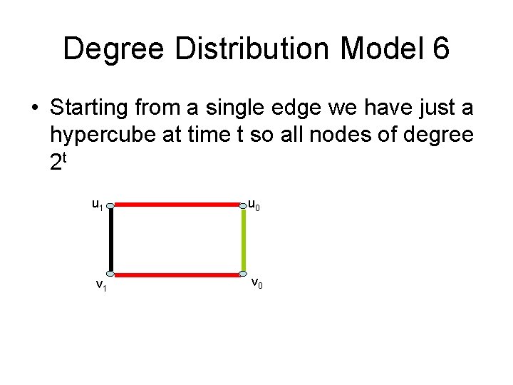
Degree Distribution Model 6 • Starting from a single edge we have just a hypercube at time t so all nodes of degree 2 t u 1 u 0 v 1 v 0

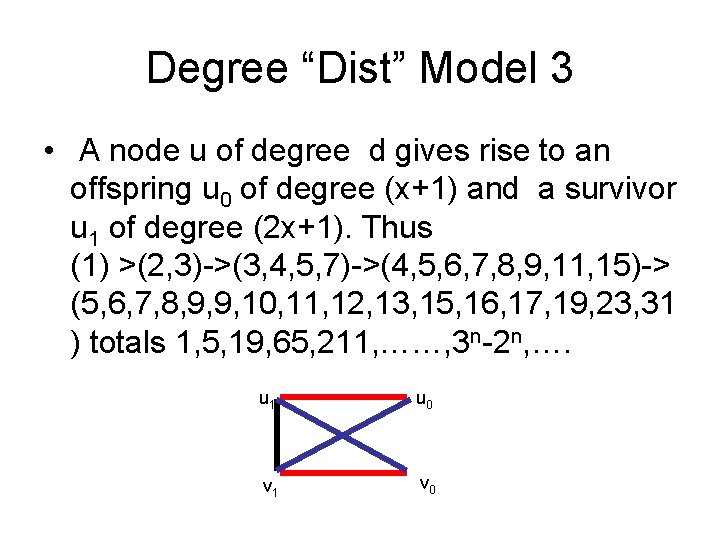
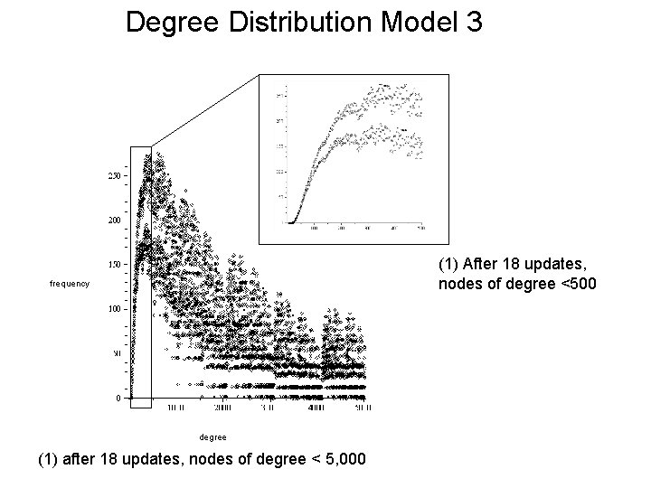
Degree “Dist” Model 3 • A node u of degree d gives rise to an offspring u 0 of degree (x+1) and a survivor u 1 of degree (2 x+1). Thus (1) >(2, 3)->(3, 4, 5, 7)->(4, 5, 6, 7, 8, 9, 11, 15)-> (5, 6, 7, 8, 9, 9, 10, 11, 12, 13, 15, 16, 17, 19, 23, 31 ) totals 1, 5, 19, 65, 211, ……, 3 n-2 n, …. u 1 u 0 v 1 v 0

Degree Distribution Model 3 (1) After 18 updates, nodes of degree <500 frequency degree (1) after 18 updates, nodes of degree < 5, 000

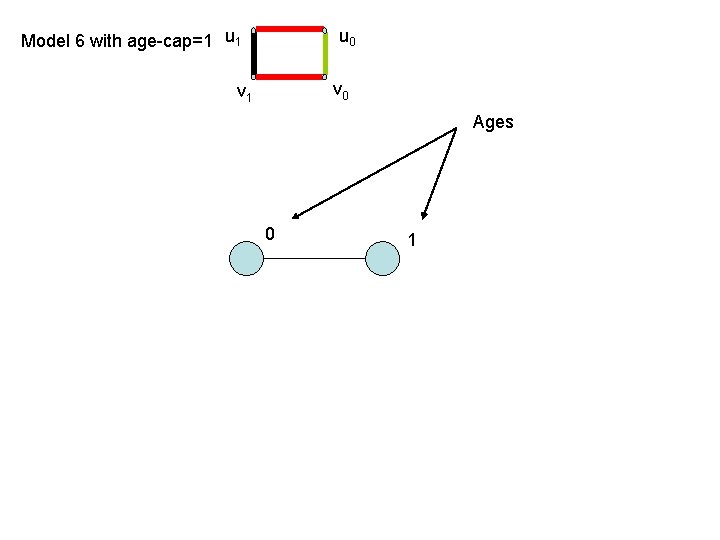
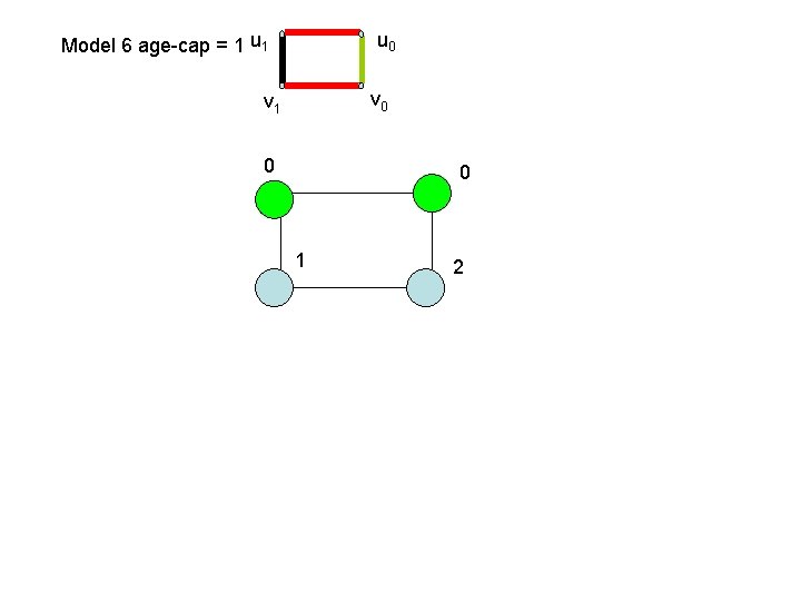
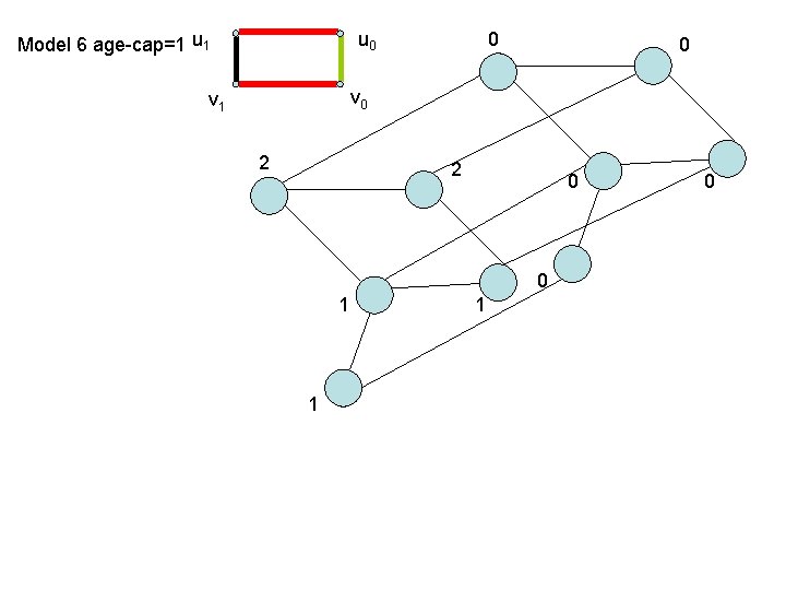
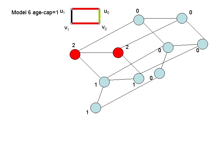
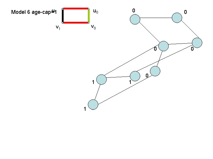
Age Culling • Suppose now that we associate with each node an index which we regard as its age. • If at time t node u in V is age s then at time t+1 u 1 is of age s+1 and u 0 is of age 0. • We suppose that after reproduction a node of age Q+1 dies (i. e. is deleted from the graph)

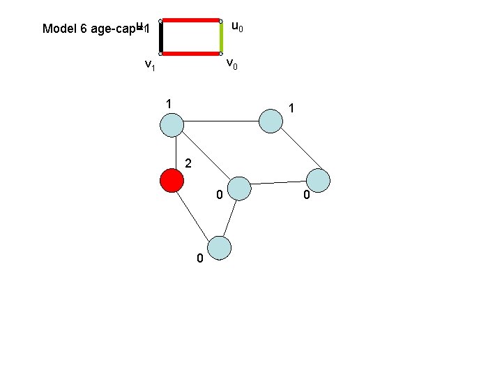
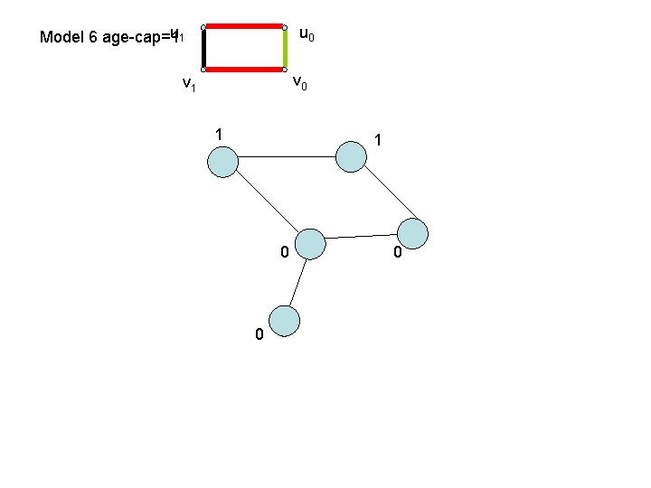
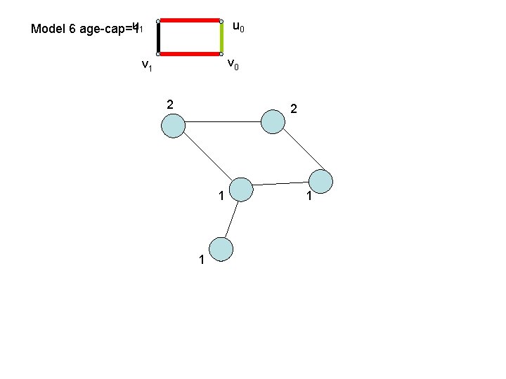
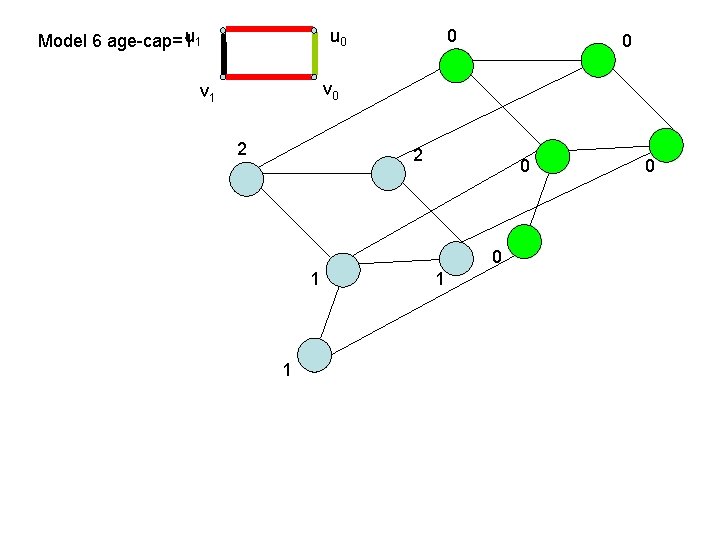
Model 6 Age Culled u 1 u 0 v 1 Grows as hypercube with pure reproduction v 0

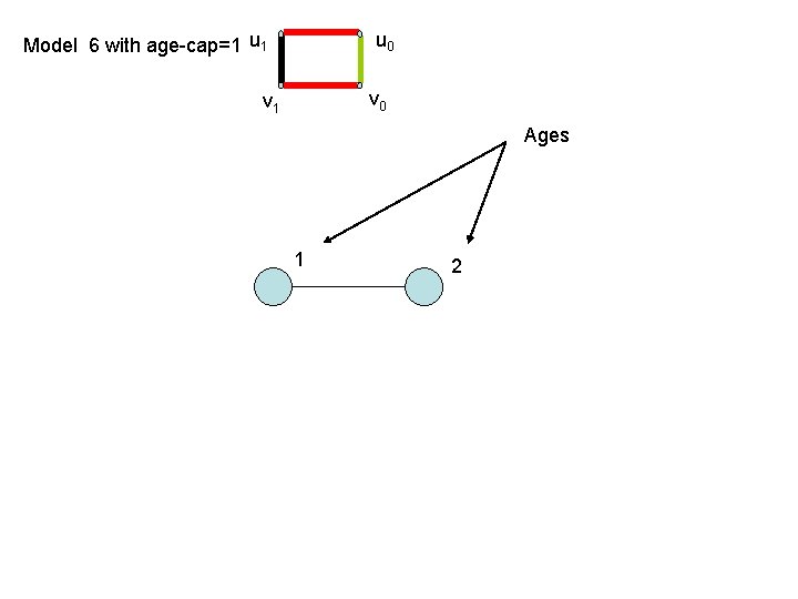
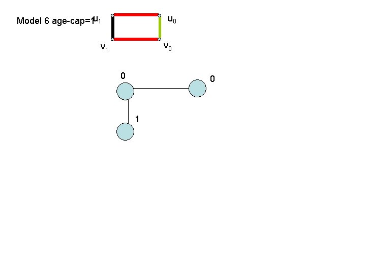
Model 6 with age-cap=1 u 0 v 1 Ages 0 1

Model 6 with age-cap=1 u 0 v 1 Ages 1 2

Model 6 age-cap = 1 u 0 v 1 0 0 1 2

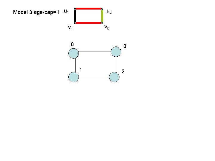
Model 3 age-cap=1 u 0 v 1 0 0 1 2

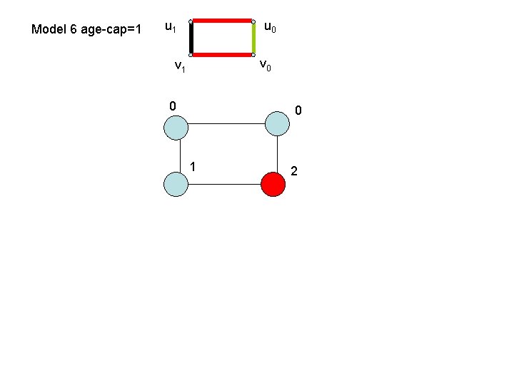
Model 6 age-cap=1 u 0 v 1 0 0 1 2

Model 6 age-cap=1 u 1 u 0 v 1 0 0 1

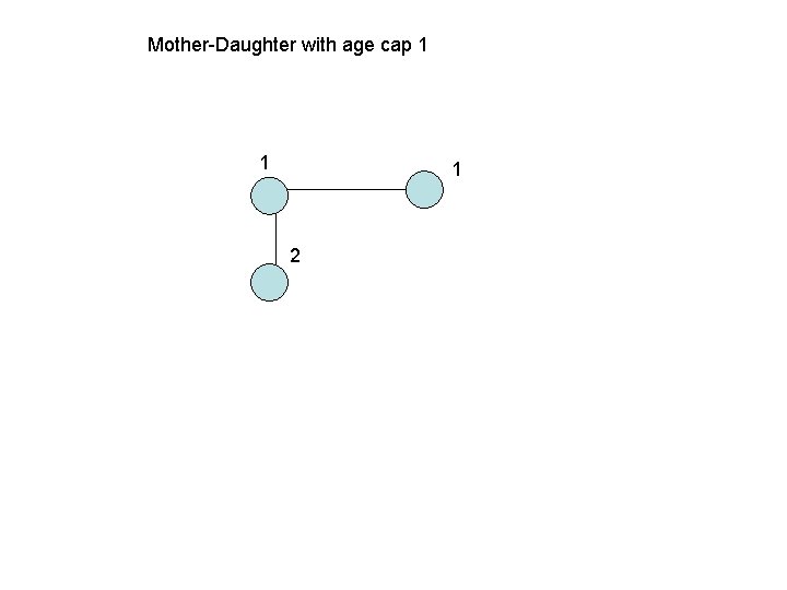
Mother-Daughter with age cap 1 1 1 2

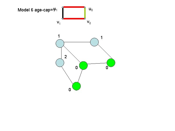
Model 6 age-cap=1 u 1 u 0 v 1 1 1 2 0 0 0

u 1 Model 6 age-cap=1 u 0 v 1 1 1 2 0 0 0

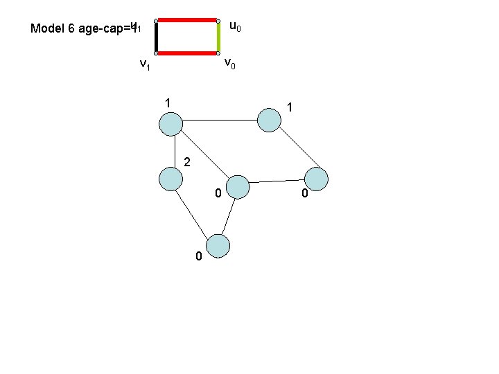
u 1 Model 6 age-cap=1 u 0 v 1 1 1 2 0 0 0

u 1 Model 6 age-cap=1 u 0 v 1 1 1 0 0 0

u 1 Model 6 age-cap=1 u 0 v 1 2 2 1 1 1

Model 6 age-cap=1 u 1 u 0 0 0 v 1 2 2 0 0 1 1 1 0

Model 6 age-cap=1 u 0 0 0 v 1 2 2 0 0 1 1 1 0

Model 6 age-cap=1 u 0 0 0 v 1 2 2 0 0 1 1 1 0

u 1 Model 6 age-cap=1 u 0 0 0 v 1 0 0 1 1 1 0

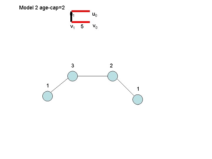
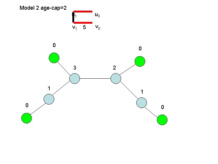
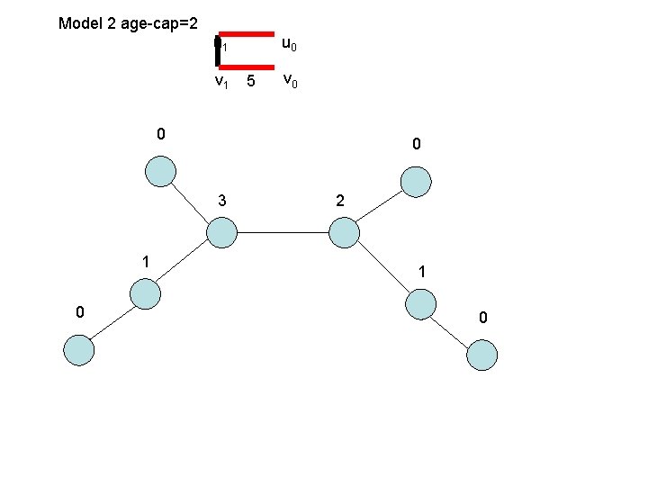
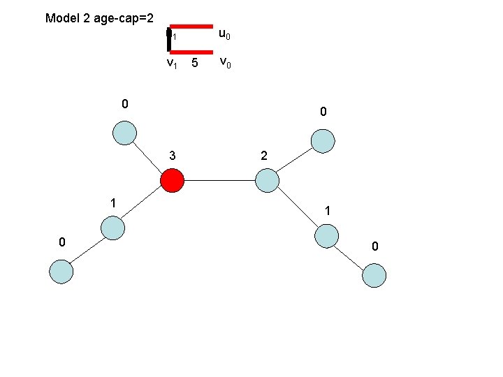
Model 2 • This is the easiest case to treat since the graph grows trees on each original individual. Here we can start with a single node

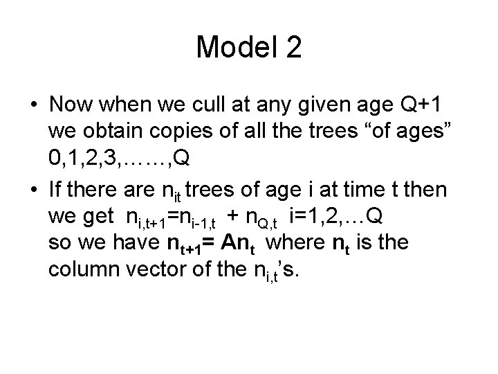
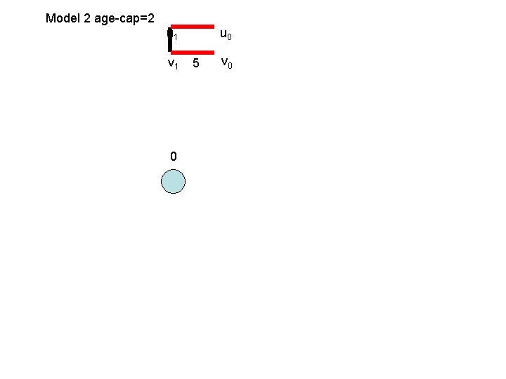
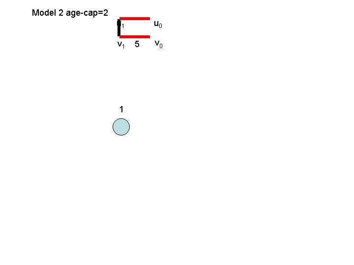
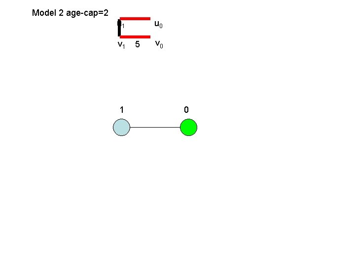
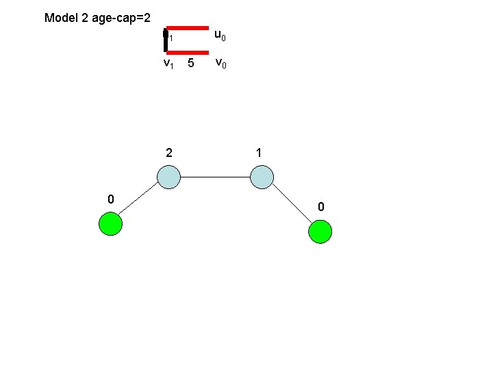
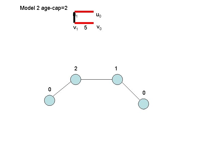
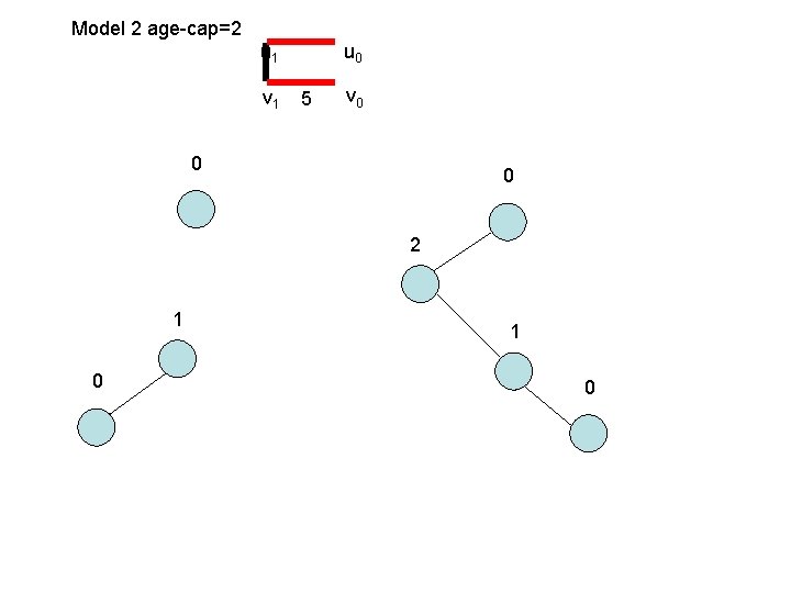
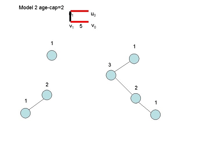
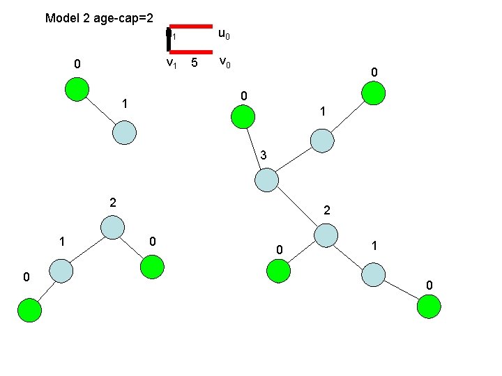
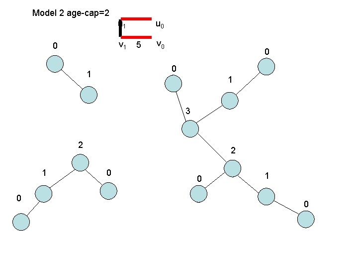
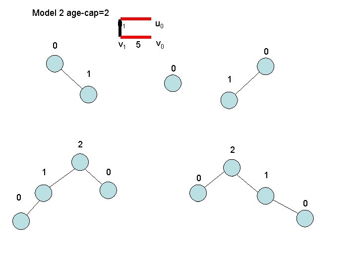
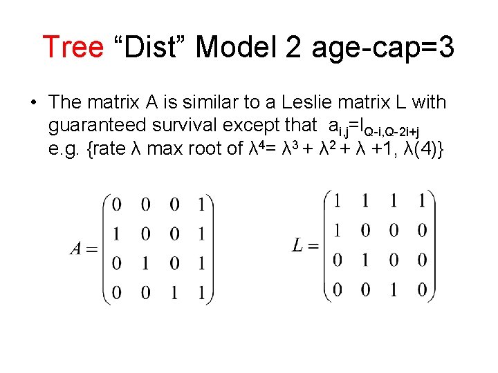
Model 2 • Now when we cull at any given age Q+1 we obtain copies of all the trees “of ages” 0, 1, 2, 3, ……, Q • If there are nit trees of age i at time t then we get ni, t+1=ni-1, t + n. Q, t i=1, 2, …Q so we have nt+1= Ant where nt is the column vector of the ni, t’s.

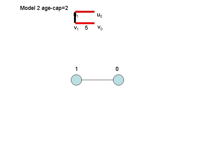
Model 2 age-cap=2 u 1 v 1 0 u 0 5 v 0

Model 2 age-cap=2 u 1 v 1 1 u 0 5 v 0

Model 2 age-cap=2 u 1 v 1 1 u 0 5 v 0 0

Model 2 age-cap=2 u 1 v 1 1 u 0 5 v 0 0

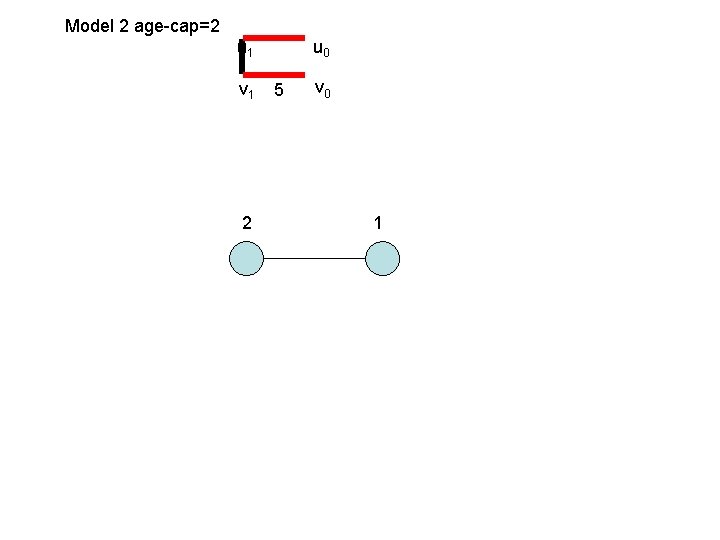
Model 2 age-cap=2 u 1 v 1 2 u 0 5 v 0 1

Model 2 age-cap=2 u 1 v 1 2 0 u 0 5 v 0 1 0

Model 2 age-cap=2 u 1 v 1 2 0 u 0 5 v 0 1 0

Model 2 age-cap=2 u 1 v 1 3 1 u 0 5 v 0 2 1

Model 2 age-cap=2 u 1 v 1 u 0 5 v 0 0 0 3 1 0 2 1 0

Model 2 age-cap=2 u 1 v 1 u 0 5 v 0 0 0 3 1 0 2 1 0

Model 2 age-cap=2 u 1 v 1 u 0 5 v 0 0 0 3 1 0 2 1 0

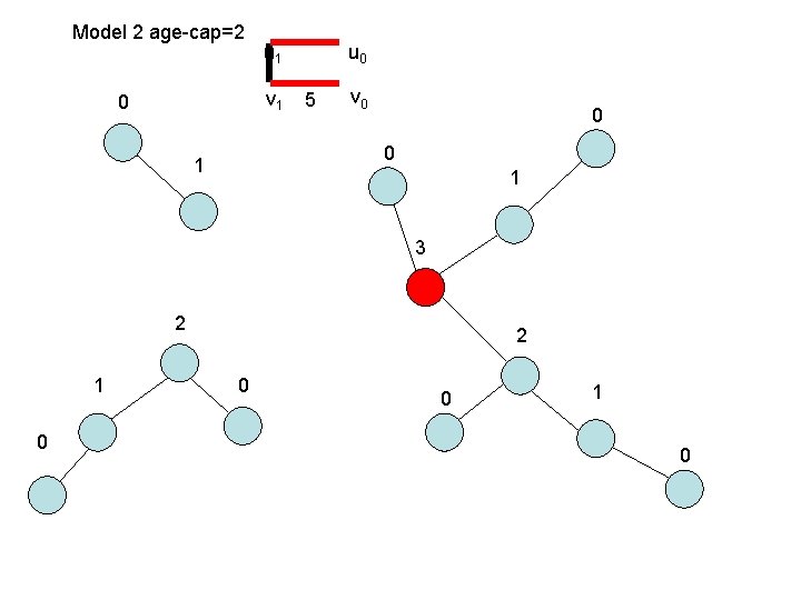
Model 2 age-cap=2 u 1 v 1 u 0 5 v 0 0 0 2 1 0

Model 2 age-cap=2 u 1 v 1 u 0 5 v 0 1 1 3 2 1

Model 2 age-cap=2 u 1 v 1 0 u 0 5 v 0 0 0 1 1 3 2 1 0 2 0 0 1 0

Model 2 age-cap=2 u 1 v 1 0 u 0 5 v 0 0 0 1 1 3 2 1 0 2 0 0 1 0

Model 2 age-cap=2 u 1 v 1 0 u 0 5 v 0 0 0 1 1 3 2 1 0 2 0 0 1 0

Model 2 age-cap=2 u 1 v 1 0 u 0 5 v 0 0 0 1 1 2 1 0 2 0 0 1 0

Tree “Dist” Model 2 age-cap=3 • The matrix A is similar to a Leslie matrix L with guaranteed survival except that ai, j=l. Q-i, Q-2 i+j e. g. {rate λ max root of λ 4= λ 3 + λ 2 + λ +1, λ(4)}

Leslie Matrix other elements all 0

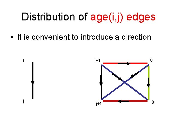
Distribution of age(i, j) edges • It is convenient to introduce a direction i j i+1 j+1 0 0

Distribution of age(i, j) edges

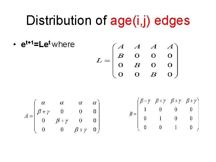
Distribution of age(i, j) edges • et+1=Let where

Distribution of age(i, j) edges • We can prove that the system is irreducible (though if α=0 need to refine the state space to exclude (i, i) states). • Essentially a generalisation of the Lesley matrix notion. • Eigenvalues related to generalisations of the “golden ratio” (tribonacci, etc. )

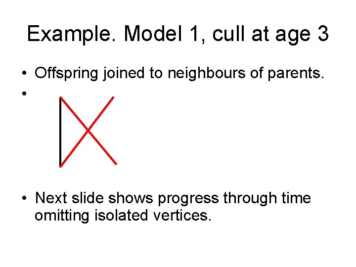
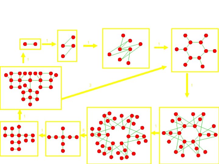
Example. Model 1, cull at age 3 • Offspring joined to neighbours of parents. • • Next slide shows progress through time omitting isolated vertices.

Degree cap = 6 1 1 3 1 1 1 6 1

References • Southwell & Cannings, Some models of graph reproduction; 1 Pure Reproduction. (to appear) AM. 2 Age Capped Vertices (to appear) AM 3 Game Based Reproduction (to appear) AM • Jordan & Southwell. Further properties of reproducing graphs (to appear) AM • AM http: //www. scirp. org/journal/am/

Applied Mathematics • Editor in Chief …. CC Editorial Board includes Mark Broom David Greenhalgh http: //www. scirp. org/journal/am/

Other Results • For age-culled, degree distribution diameter average distance

Further Work • 1) Culling by degree • 2) Stochastic/non-synchronous • 3) Conflict with neighbours to determine survivor &/or reproduction