REPEATED MEASURES ANOVA Repeated Measures ANOVA A repeated

REPEATED MEASURES ANOVA

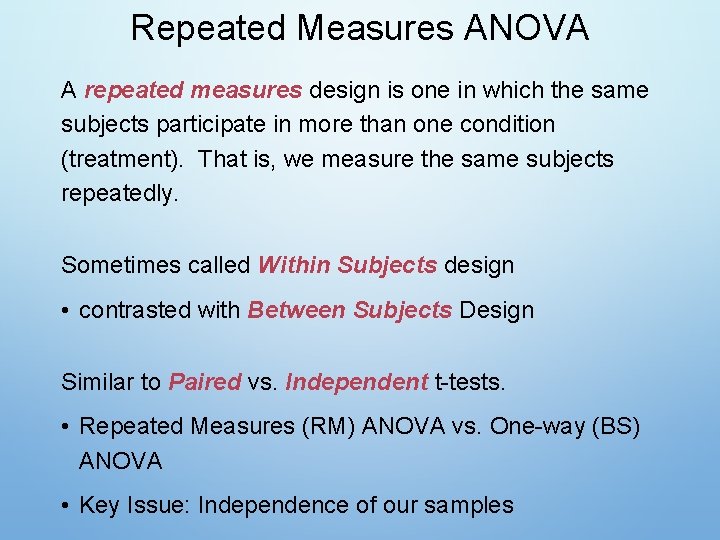
Repeated Measures ANOVA A repeated measures design is one in which the same subjects participate in more than one condition (treatment). That is, we measure the same subjects repeatedly. Sometimes called Within Subjects design • contrasted with Between Subjects Design Similar to Paired vs. Independent t-tests. • Repeated Measures (RM) ANOVA vs. One-way (BS) ANOVA • Key Issue: Independence of our samples

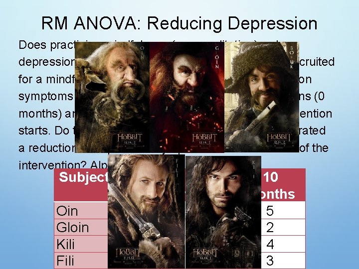
RM ANOVA: Reducing Depression Does practicing mindfulness (e. g. meditation) reduce depression symptoms? A group of participants are recruited for a mindfulness intervention. Their level of depression symptoms are measured before the intervention begins (0 months) and 5 months and 10 months after the intervention starts. Do the data suggest that participants demonstrated a reduction in depression symptoms over the course of the intervention? Alpha=. 05 Subject Oin Gloin Kili Fili 0 5 months 6 5 5 5 6 4 5 4 10 months 5 2 4 3

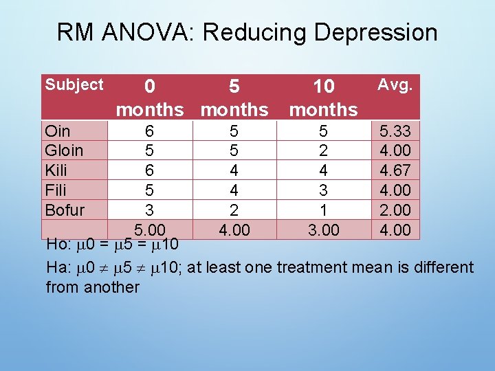
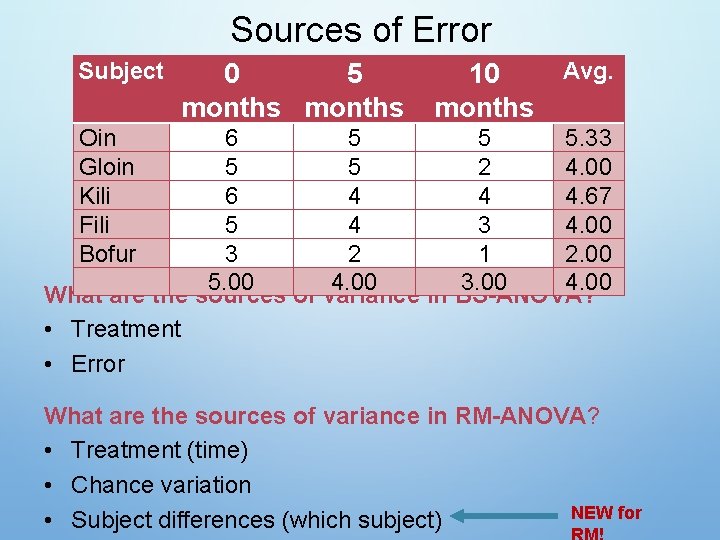
RM ANOVA: Reducing Depression Subject Oin Gloin Kili Fili Bofur 0 5 months Avg. 10 months 6 5 5 5. 33 5 5 2 4. 00 6 4 4 4. 67 5 4 3 4. 00 3 2 1 2. 00 5. 00 4. 00 3. 00 4. 00 Ho: 0 = 5 = 10 Ha: 0 5 10; at least one treatment mean is different from another

Sources of Error Subject 0 5 months Avg. 10 months Oin Gloin Kili Fili Bofur 6 5 5 5. 33 5 5 2 4. 00 6 4 4 4. 67 5 4 3 4. 00 3 2 1 2. 00 5. 00 4. 00 3. 00 4. 00 What are the sources of variance in BS-ANOVA? • Treatment • Error What are the sources of variance in RM-ANOVA? • Treatment (time) • Chance variation NEW for • Subject differences (which subject)

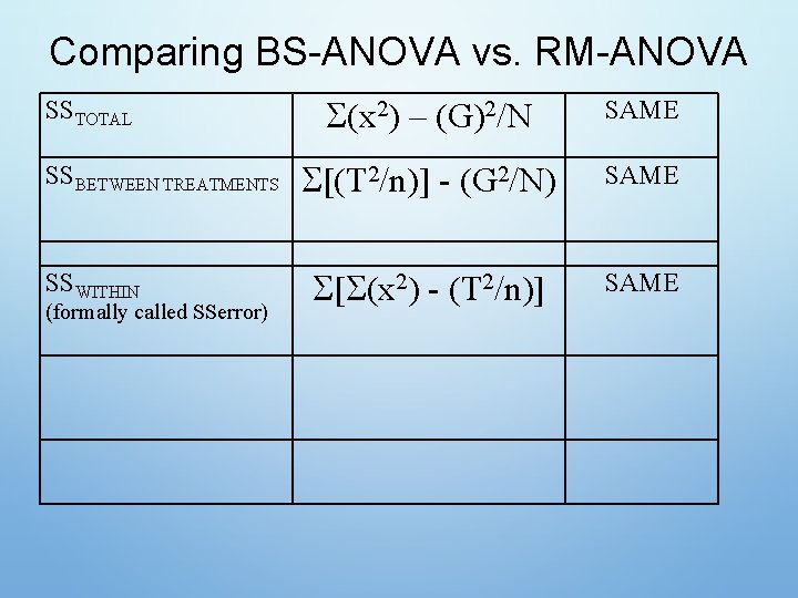
Comparing BS-ANOVA vs. RM-ANOVA SSTOTAL SSBETWEEN TREATMENTS SSWITHIN (formally called SSerror) (x 2) – (G)2/N SAME [(T 2/n)] - (G 2/N) SAME [ (x 2) - (T 2/n)] SAME

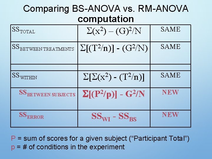
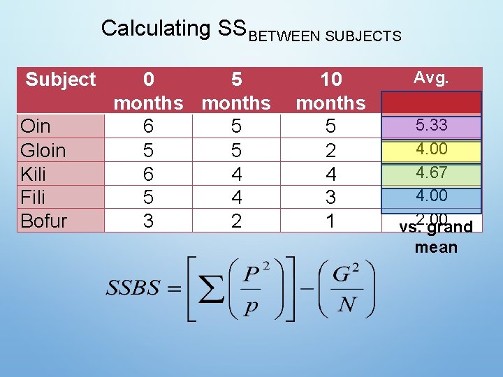
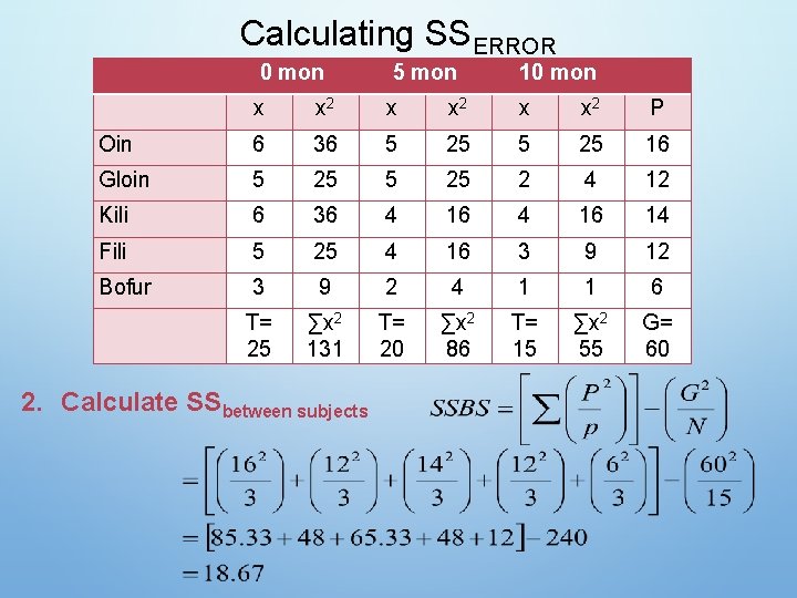
Comparing BS-ANOVA vs. RM-ANOVA computation SSTOTAL SAME (x 2) – (G)2/N SSBETWEEN TREATMENTS SSWITHIN SSBETWEEN SUBJECTS SSERROR [(T 2/n)] - (G 2/N) SAME [ (x 2) - (T 2/n)] SAME [(P 2/p)] - G 2/N NEW SSWI - SSBS NEW P = sum of scores for a given subject (“Participant Total”) p = # of conditions in the experiment

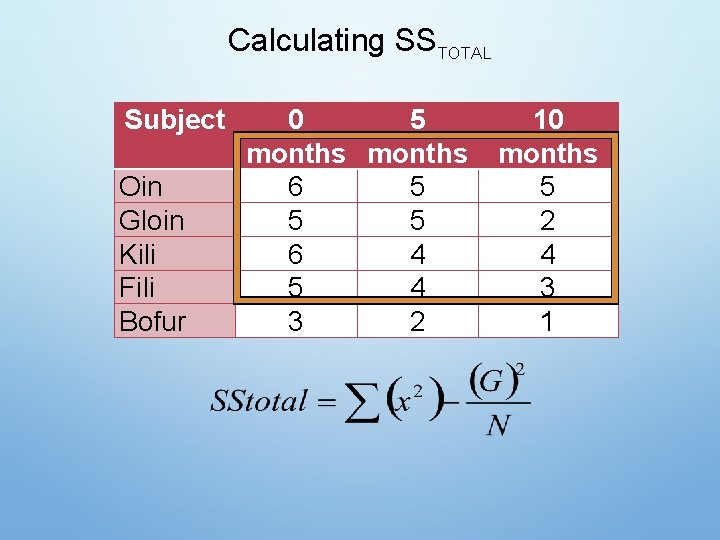
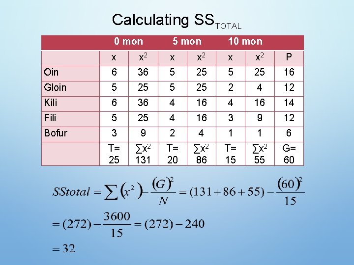
Calculating SSTOTAL Subject Oin Gloin Kili Fili Bofur 0 5 months 6 5 5 5 6 4 5 4 3 2 10 months 5 2 4 3 1

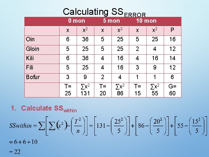
Calculating SSTOTAL 0 mon 5 mon 10 mon x x 2 P Oin 6 36 5 25 16 Gloin 5 25 2 4 12 Kili 6 36 4 16 14 Fili 5 25 4 16 3 9 12 Bofur 3 9 2 4 1 1 6 T= 25 ∑x 2 131 T= 20 ∑x 2 86 T= 15 ∑x 2 55 G= 60

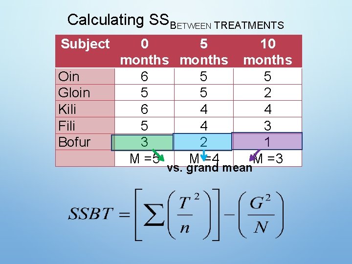
Calculating SSBETWEEN TREATMENTS Subject Oin Gloin Kili Fili Bofur 0 5 months 6 5 5 5 6 4 5 4 3 2 M =5 M =4 10 months 5 2 4 3 1 M =3 vs. grand mean

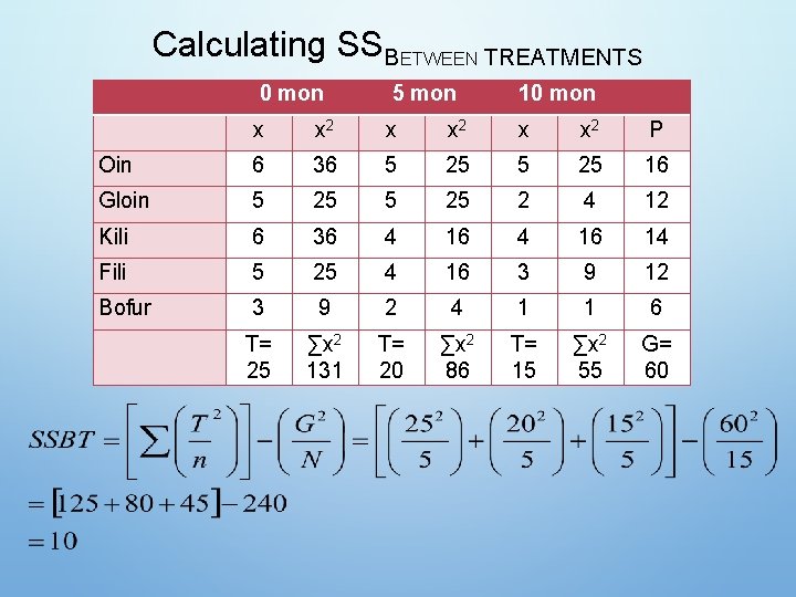
Calculating SSBETWEEN TREATMENTS 0 mon 5 mon 10 mon x x 2 P Oin 6 36 5 25 16 Gloin 5 25 2 4 12 Kili 6 36 4 16 14 Fili 5 25 4 16 3 9 12 Bofur 3 9 2 4 1 1 6 T= 25 ∑x 2 131 T= 20 ∑x 2 86 T= 15 ∑x 2 55 G= 60

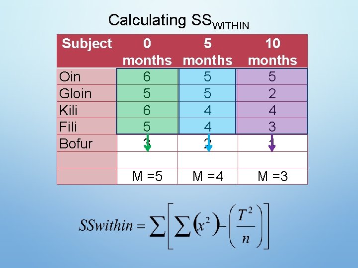
Calculating SSWITHIN Subject Oin Gloin Kili Fili Bofur 0 5 months 6 5 5 5 6 4 5 4 3 2 M =5 M =4 10 months 5 2 4 3 1 M =3

Calculating SSERROR 0 mon 5 mon 10 mon x x 2 P Oin 6 36 5 25 16 Gloin 5 25 2 4 12 Kili 6 36 4 16 14 Fili 5 25 4 16 3 9 12 Bofur 3 9 2 4 1 1 6 T= 25 ∑x 2 131 T= 20 ∑x 2 86 T= 15 ∑x 2 55 G= 60 1. Calculate SSwithin

Calculating SSBETWEEN SUBJECTS Subject Oin Gloin Kili Fili Bofur 0 5 months 6 5 5 5 6 4 5 4 3 2 10 months 5 2 4 3 1 Avg. 5. 33 4. 00 4. 67 4. 00 vs. 2. 00 grand mean

Calculating SSERROR 0 mon 5 mon 10 mon x x 2 P Oin 6 36 5 25 16 Gloin 5 25 2 4 12 Kili 6 36 4 16 14 Fili 5 25 4 16 3 9 12 Bofur 3 9 2 4 1 1 6 T= 25 ∑x 2 131 T= 20 ∑x 2 86 T= 15 ∑x 2 55 G= 60 2. Calculate SSbetween subjects

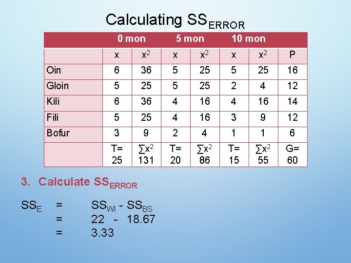
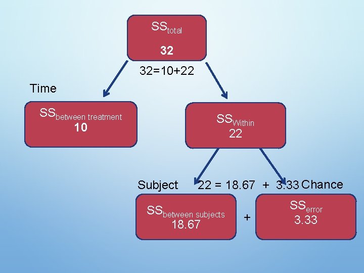
Calculating SSERROR 0 mon 5 mon 10 mon x x 2 P Oin 6 36 5 25 16 Gloin 5 25 2 4 12 Kili 6 36 4 16 14 Fili 5 25 4 16 3 9 12 Bofur 3 9 2 4 1 1 6 T= 25 ∑x 2 131 T= 20 ∑x 2 86 T= 15 ∑x 2 55 G= 60 3. Calculate SSERROR SSE = = = SSWI - SSBS 22 - 18. 67 3. 33

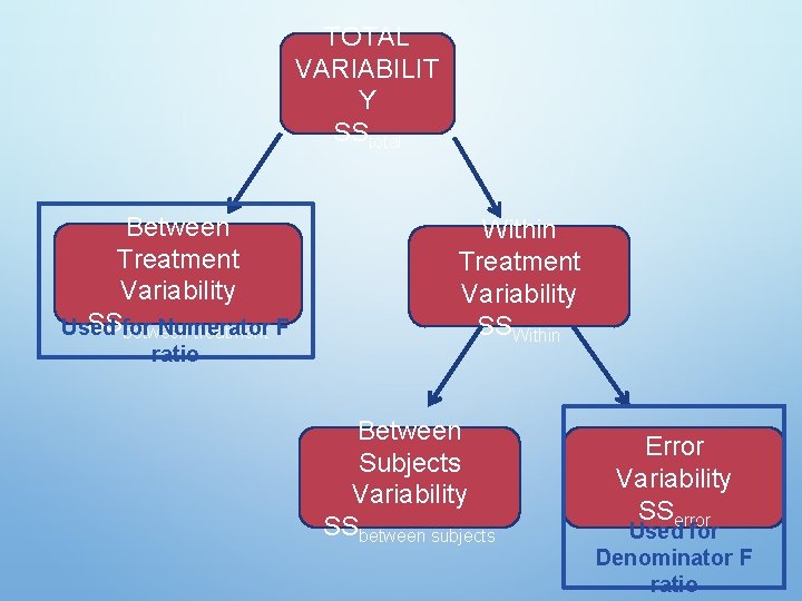
TOTAL VARIABILIT Y SStotal Between Treatment Variability SSfor Used Numerator between treatment F ratio Within Treatment Variability SSWithin Between Subjects Variability SSbetween subjects Error Variability SSerror Used for Denominator F ratio

SStotal 32 32=10+22 Time SSbetween treatment 10 SSWithin 22 Subject 22 = 18. 67 + 3. 33 Chance SSbetween subjects 18. 67 + SSerror 3. 33

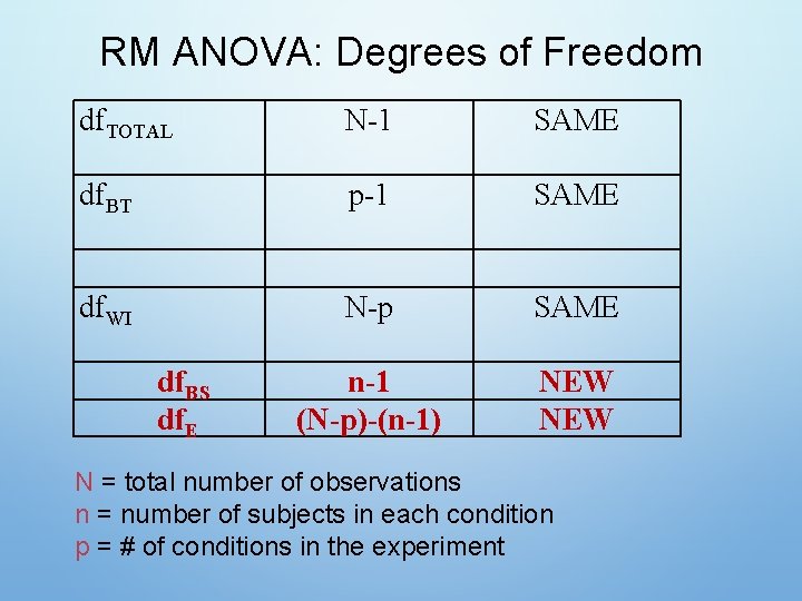
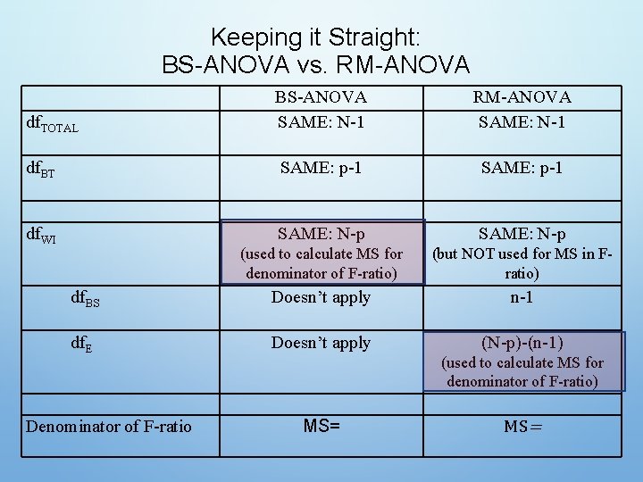
RM ANOVA: Degrees of Freedom df. TOTAL N-1 SAME df. BT p-1 SAME df. WI N-p SAME n-1 (N-p)-(n-1) NEW df. BS df. E N = total number of observations n = number of subjects in each condition p = # of conditions in the experiment

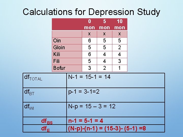
Calculations for Depression Study Oin Gloin Kili Fili Bofur 0 5 10 mon mon x x x 6 5 5 2 6 4 4 5 4 3 3 2 1 df. TOTAL N-1 = 15 -1 = 14 df. BT p-1 = 3 -1=2 df. WI N-p = 15 – 3 = 12 df. BS df. E n-1 = 5 -1 = 4 (N-p)-(n-1) = (15 -3)- (5 -1) =8

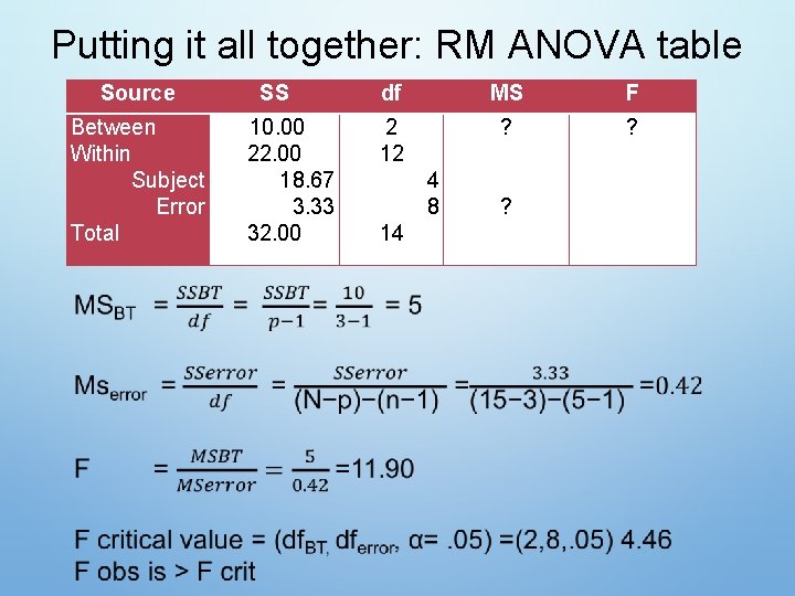
Putting it all together: RM ANOVA table Source Between Within Subject Error Total SS 10. 00 22. 00 18. 67 3. 33 32. 00 df MS F 2 12 ? ? 4 8 14 ?

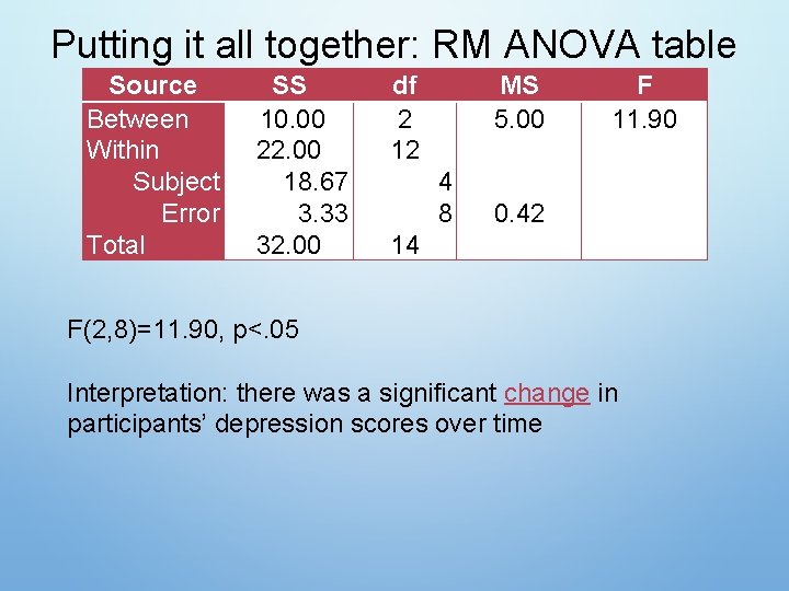
Putting it all together: RM ANOVA table Source Between Within Subject Error Total SS 10. 00 22. 00 18. 67 3. 33 32. 00 df 2 12 MS 5. 00 4 8 F 11. 90 0. 42 14 F(2, 8)=11. 90, p<. 05 Interpretation: there was a significant change in participants’ depression scores over time

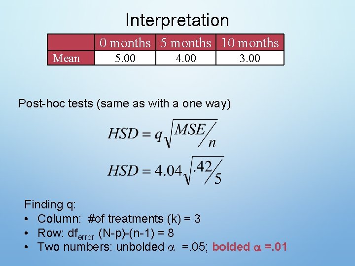
Interpretation 0 months 5 months 10 months Mean 5. 00 4. 00 3. 00 Post-hoc tests (same as with a one way) Finding q: • Column: #of treatments (k) = 3 • Row: dferror (N-p)-(n-1) = 8 • Two numbers: unbolded =. 05; bolded =. 01

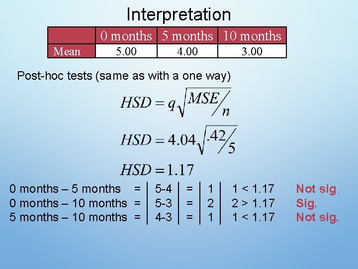
Interpretation 0 months 5 months 10 months Mean 5. 00 4. 00 3. 00 Post-hoc tests (same as with a one way) 0 months – 5 months = │ 5 -4 │ = │ 1 < 1. 17 0 months – 10 months = │ 5 -3 │ = │ 2 > 1. 17 5 months – 10 months = │ 4 -3 │ = │ 1 < 1. 17 Not sig. Sig. Not sig.

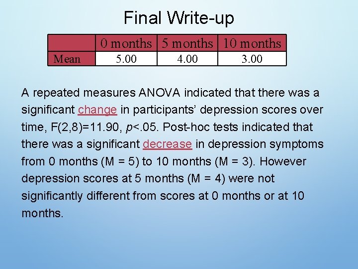
Final Write-up 0 months 5 months 10 months Mean 5. 00 4. 00 3. 00 A repeated measures ANOVA indicated that there was a significant change in participants’ depression scores over time, F(2, 8)=11. 90, p<. 05. Post-hoc tests indicated that there was a significant decrease in depression symptoms from 0 months (M = 5) to 10 months (M = 3). However depression scores at 5 months (M = 4) were not significantly different from scores at 0 months or at 10 months.

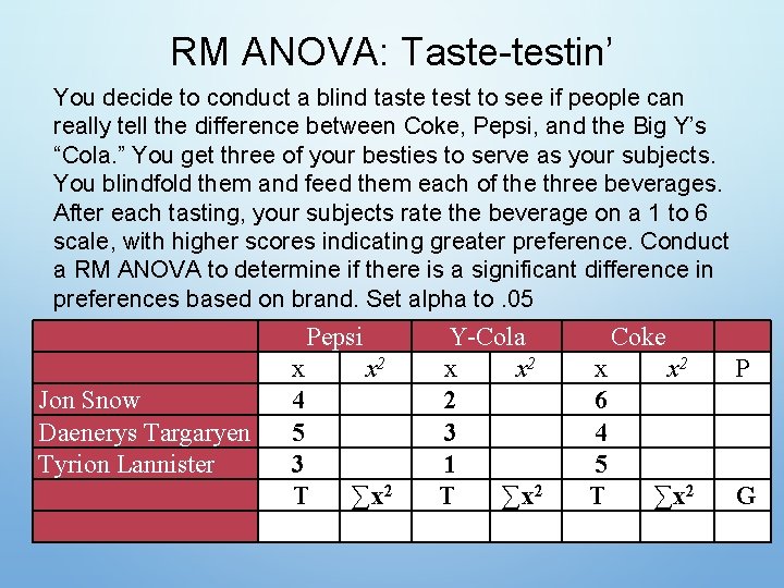
RM ANOVA: Taste-testin’ You decide to conduct a blind taste test to see if people can really tell the difference between Coke, Pepsi, and the Big Y’s “Cola. ” You get three of your besties to serve as your subjects. You blindfold them and feed them each of the three beverages. After each tasting, your subjects rate the beverage on a 1 to 6 scale, with higher scores indicating greater preference. Conduct a RM ANOVA to determine if there is a significant difference in preferences based on brand. Set alpha to. 05 Pepsi Jon Snow Daenerys Targaryen Tyrion Lannister x 4 5 3 T x 2 ∑x 2 Y-Cola x x 2 2 3 1 T ∑x 2 Coke x 6 4 5 T x 2 P ∑x 2 G

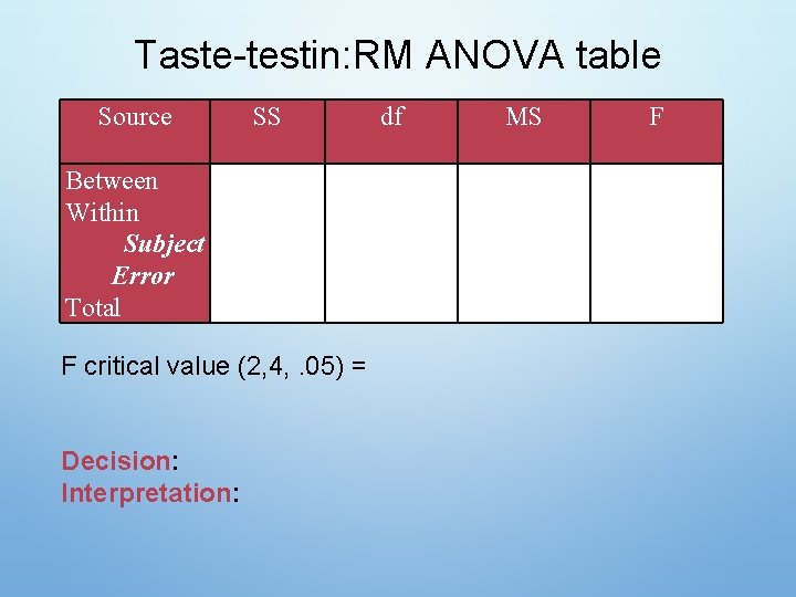
Taste-testin: RM ANOVA table Source SS Between Within Subject Error Total F critical value (2, 4, . 05) = Decision: Interpretation: df MS F

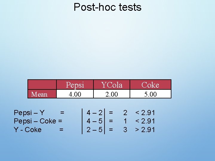
Post-hoc tests Mean Pepsi – Y = Pepsi – Coke = Y - Coke = Pepsi YCola Coke 4. 00 2. 00 5. 00 │ 4 – 2│ = │ 4 – 5│ = │ 2 – 5│ = 2 1 3 < 2. 91 > 2. 91

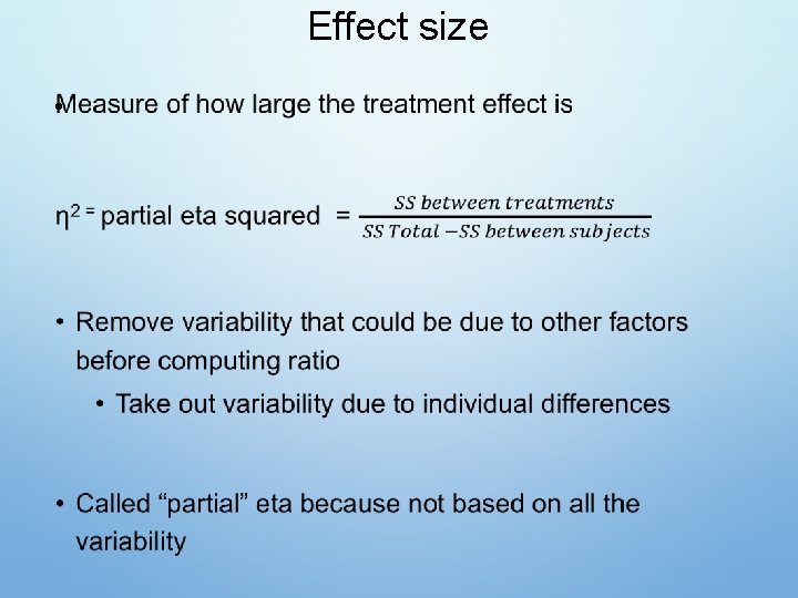
Effect size •

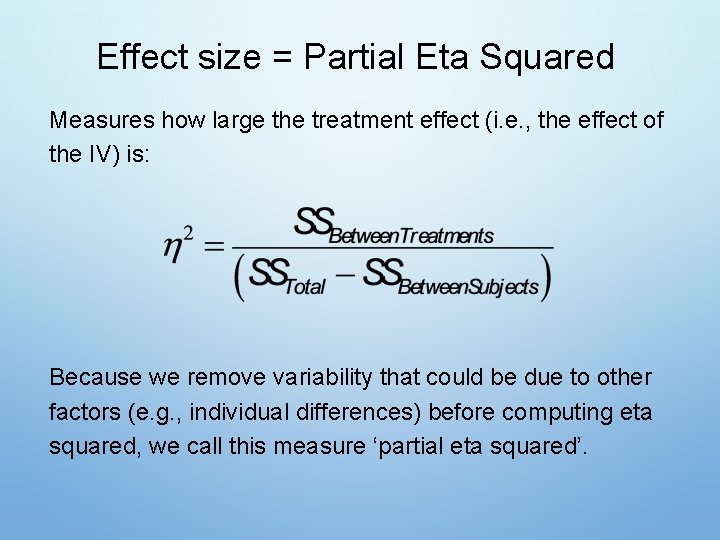
Effect size = Partial Eta Squared Measures how large the treatment effect (i. e. , the effect of the IV) is: Because we remove variability that could be due to other factors (e. g. , individual differences) before computing eta squared, we call this measure ‘partial eta squared’.

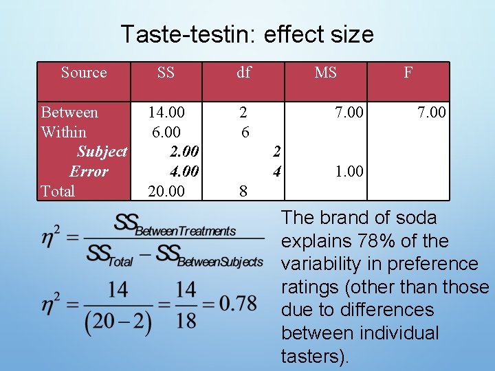
Taste-testin: effect size Source Between Within Subject Error Total SS 14. 00 6. 00 2. 00 4. 00 20. 00 df MS 2 6 7. 00 2 4 F 7. 00 1. 00 8 The brand of soda explains 78% of the variability in preference ratings (other than those due to differences between individual tasters).

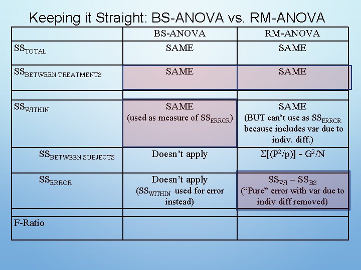
Keeping it Straight: BS-ANOVA vs. RM-ANOVA BS-ANOVA SAME RM-ANOVA SAME SSBETWEEN TREATMENTS SAME SSWITHIN SAME (used as measure of SSERROR) (BUT can’t use as SSERROR because includes var due to indiv. diff. ) SSBETWEEN SUBJECTS Doesn’t apply [(P 2/p)] - G 2/N SSERROR Doesn’t apply SSWI – SSBS SSTOTAL F-Ratio (SSWITHIN used for error instead) (“Pure” error with var due to indiv diff removed)

Keeping it Straight: BS-ANOVA vs. RM-ANOVA df. TOTAL BS-ANOVA SAME: N-1 RM-ANOVA SAME: N-1 df. BT SAME: p-1 df. WI SAME: N-p (used to calculate MS for denominator of F-ratio) (but NOT used for MS in Fratio) df. BS Doesn’t apply n-1 df. E Doesn’t apply (N-p)-(n-1) Denominator of F-ratio (used to calculate MS for denominator of F-ratio) MS=